Artificial Intelligence
Shortcut to this page: ntrllog.netlify.app/ai
Info provided by Artificial Intelligence: A Modern Approach and Professor Francisco Guzman (CSULA)
What is AI?
Well, it kinda depends on what we think makes a machine "intelligent". Is it the ability for the machine to act like a human? Or is it the ability for the machine to always do the mathematically-optimal thing? And is intelligence a way of thinking or a way of behaving? These are the four main dimensions that researchers are using to think about AI.
Acting humanly: The Turing test approach
Let's say we ask a question to a computer and some people and get back their responses. If we can't tell whether the responses came from a person or from a computer, then the computer passes the Turing test.
In order to pass the Turing test, a computer would need:
- natural language processing: communicate in a human language
- knowledge representation: store what it knows or hears
- automated reasoning: answer questions and draw new conclusions
- machine learning: adapt to new circumstances and detect and extrapolate patterns
There's also a total Turing test, which tests if a computer can physically behave like a human. To pass the total test, a computer would also need:
- computer vision and speech recognition
- robotics: manipulate objects and move around
Thinking humanly: The cognitive modeling approach
While the Turing test is just focused on the computer's results, some people are more interested in the computer's process. When performing a task, does a computer go through the same thought process as a human would?
If the input-output behavior matches human behavior, then that could give us some insight into how our brains work.
We can learn about how humans think by:
- introspection: thinking about our thoughts as they go by
- psychological experiments: observing a person in action
- brain imaging: observing the brain in action
Cognitive science combines computer models and experimental techniques from psychology to study the human mind.
Thinking rationally: The "laws of thought" approach
The world of logic is pretty much, "if these statements are true, then this has to be true". If we give a computer some assumptions, can it reason its way to a correct conclusion?
In things like chess and math, all the rules are known, so it's relatively easy to make logical choices and statements. But in the real world, there's a lot of uncertainty. Interestingly, the theory of probability allows for rigorous reasoning with uncertain information. With this, we can use raw perceptual information to understand how the world works and make predictions.
Acting rationally: The rational agent approach
A computer agent is defined to be something that can operate autonomously, perceive their environment, persist over a prolonged time period, adapt to change, and create and pursue goals. A rational agent acts to achieve the best outcome.
There's a subtle distinction between "thinking" rationally and "acting" rationally. Thinking rationally is about making correct inferences. (What's implied here is that there is some (slow) deliberate reasoning process involved.) But it's possible to act rationally without having to make inferences. For example, recoiling from a hot stove, which is more of a reflex action than something you come to a conclusion about.
The rational agent approach is how most researchers approach studying AI. This is because rationality (as opposed to humanity) is easier to approach scientifically, and the rational agent approach kinda encapsulates all the other approaches. For example, in order to act rationally, a computer needs the skills that is required for it to act like a human.
So AI is the science of making machines act rationally, a.k.a. doing the right thing. The "right" thing is specified by us to the agent as an objective that it should complete. This way of thinking about AI is considered the standard model.
Beneficial machines
But the problem with the standard model is that it only works when the objective is fully specified. In the real world, it's hard to specify a goal that is complete and correct. For example, if the primary goal of a self-driving car is safety, then, of course, it's safest to just not leave the house at all, but that's not helpful; there needs to be some tradeoff. Inherently, there is a value alignment problem: the values put into the machine must be aligned with our values. That is, the machine's job shouldn't be to just complete its objective; it should also consider the costs, consequences, and benefits that would affect us.
Agents and Environments
A little more formally, an agent perceives its environment through sensors and acts upon that environment through actuators. Its percept sequence is the complete history of everything it has ever perceived. The agent looks at its percept sequence (and its built-in knowledge) to determine what action to take.
Mathematically, an agent's behavior is defined by an agent function, which maps a percept sequence to an action.
Let's take a look at a robotic vacuum cleaner. Suppose the floor is divided into two squares `A` and `B`, and that the vacuum cleaner is on square `A`. We can create a table that (theoretically) lists all the percept sequences and the actions that (we think) should be taken for each one.
| Percept sequence | Action |
|---|---|
| Square `A` is clean | Move right |
| Square `A` is dirty | Clean |
| Square `B` is clean | Move left |
| Square `B` is dirty | Clean |
| Square `A` is clean, Square `A` is clean | Move right |
| Square `A` is clean, Square `A` is dirty | Clean |
| `vdots` | `vdots` |
| Square `A` is clean, Square `A` is clean, Square `A` is clean | Move right |
| Square `A` is clean, Square `A` is clean, Square `A` is dirty | Clean |
| `vdots` | `vdots` |
In this very simplified scenario, it's pretty easy to see what the right actions should be. But in general, it's a bit harder to know what the correct action should be.
Good Behavior: The Concept of Rationality
So how can we know what the "right" action should be? How do we know that an action is "right"?
Performance Measures
Generally, we assess how good an agent is by the consequences of its actions (consequentialism). If the resulting environment is desirable, then the agent is good. (good bot)
A performance measure is a way to evaluate the agent's behavior in an environment. We have to be a little bit thoughtful about how we come up with a performance measure though. For the vacuum cleaner, it might sound like a good idea to measure performance by how much dirt is cleaned up in an eight-hour shift. The problem with this is that a rational agent would maximize performance by repeatedly cleaning up the dirt and dumping it on the floor. A better performance measure would be to reward the agent for a clean floor. For example, we could give it one point for each clean square, incentivizing it to maximize the number of points (and thus the number of clean squares).
As we can see, it's better to come up with performance measures based on what we want to be achieved in the environment, rather than what we think the agent should do.
Rationality
Formally, for each possible percept sequence, a rational agent should use the evidence provided by the percept sequence and its built-in knowledge to select an action that maximizes its performance measure (definition of a rational agent). We can assess whether an agent is rational by looking at four things:
- the performance measure that defines success
- the agent's prior knowledge of the environment
- the actions that the agent can perform
- the agent's percept sequence to date
For our vacuum cleaner:
- the performance measure awards one point for each clean square
- the "geography" of the environment is known (but not the dirt distribution)
- the actions are moving right, moving left, and cleaning
- the agent's percept sequence consists of what square it's at and whether it's clean
Under these circumstances, we can expect our vacuum cleaner to do at least as well as any other agent.
Suppose that we change the performance measure to deduct one point for each movement. Once all the squares are clean, the vacuum cleaner will just keep moving back and forth (we never defined "stopping" as an action). Then it would be irrational.
Omniscience, learning, and autonomy
One thing that's been sorta glossed over is that the agent doesn't know what will actually happen if it performs an action, i.e., it's not omniscient. So it's more correct to say that a rational agent tries to maximize expected performance.
In order to be able to maximize expected performance, the agent needs to be able to gather information and learn.
Crossing a street when it's empty is rational. It's expected that you'll reach the other side. But if you get hit by a car because you didn't look before crossing... well... then that's not rational.
If an agent only relies on its built-in knowledge, then it lacks autonomy. In order to be autonomous, the agent should build on its existing knowledge by learning. By being able to learn, a rational agent can be expected to succeed in a variety of environments.
The Nature of Environments
A task environment is the problem that we are trying to solve by using a rational agent.
Specifying the task environment
We can specify a task environment by specifying the performance measure, the environment, and the agent's actuators and sensors (PEAS). Yes, these are the four things we listed out when defining how an agent can be rational. The vacuum cleaner example was fairly simple though, so we can look at something more complicated, like an automated taxi.
- performance measure: correct destination, minimize fuel consumption, minimize time/cost, minimize impact on other drivers, maximize passenger safety and comfort, maximize profits
- environment: roads, traffic, obstacles, police, pedestrians, passengers, weather
- actuators: steering, accelerator, brake, signal, horn, display screen, speech
- sensors: cameras, speedometer, GPS, accelerometer, radar, microphone, touchscreen
Properties of task environments
A task environment can be fully observable or partially observable. If the agent's sensors give it access to the complete state of the environment, then the task environment is fully observable. Noisy and inaccurate sensors would make it partially observable. Or maybe the capability simply isn't available. For example, a vacuum with a local sensor can't tell whether there is dirt in other squares and an automated taxi can't know what other drivers are thinking. Basically, if the agent has to make a guess, then the environment is partially observable.
An environment can also be unobservable if the agent has no sensors.
A task environment can be single-agent or multiagent. This one's pretty self-explanatory.
Though there is a small subtlety. Does an automated taxi have to view another car as another agent or can it think of it as just another "object"? The answer depends on whether the "object's" performance measure is affected by the automated taxi. If it is, then it must be viewed as an agent.
A multiagent environment can be competitive or cooperative. In a competitive environment, maximizing/improving one agent's performance measure minimizes/worsens another agent's performance measure. In a cooperative environment, all agents' performance measures can be maximized.
A task environment can be deterministic or nondeterministic. If the next state of the environment is completely determined by the current state and the agent's action, then it is deterministic. If something unpredictable can happen, then it is nondeterministic. For example, driving is nondeterministic because traffic cannot be predicted exactly. But if you want to argue that traffic is predictable, then some more reasons that driving is nondeterministic are that the tires may blow out unexpectedly or that the engine may seize up unexpectedly.
A stochastic environment is a nondeterministic environment that deals with probabilities. "There's a `25%` chance of rain" is stochastic, while "There's a chance of rain" is nondeterministic.
A task environment can be episodic or sequential. Classifying images is episodic because classifying the current image doesn't depend on the decisions for past images nor does it affect the decisions of future images. Chess and driving are sequential because the available moves depend on past moves, and the next move affects future moves.
A task environment can be static or dynamic. A static environment doesn't change while the agent is deciding on its next action, whereas a dynamic one does. Driving is dynamic because the other cars are always moving. Chess is static. As time passes, if the environment doesn't change, but the agent's performance score does, then the environment is semidynamic. Timed chess is semidynamic.
A task environment can be discrete or continuous. This refers to the state of the environment, the way time is handled, and the percepts and actions of the agent. Chess has a finite number of distinct states, percepts, and actions, which means it is discrete. Whereas in driving, speed and location range over continuous values.
A task environment can be known or unknown. (Well, strictly speaking, not really.) This is not referring to the environment itself, but to the agent's knowledge about the rules of its environment. In a known environment, the outcomes (or outcome probabilities) for all actions are given.
Known vs unknown is not the same as fully vs partially observable. A known environment can be partially observable, like solitaire, where we know the rules, but we can't see the cards that are turned over. An unknown environment can be fully observable, like a new video game, where the screen shows the entire game state, but we don't know what the buttons do yet until we try them.
The hardest case is partially observable, multiagent, nondeterministic, sequential, dynamic, continuous, and unknown. Driving is all of these, except the environment is known.
The Structure of Agents
Now we get to go over the more technical aspects of how agents work.
Recall that an agent function maps percept sequences to actions. An agent program is code that implements the agent function. This program runs on some sort of computing device with sensors and actuators, referred to as the agent architecture.
agent = architecture + program
In general, the architecture makes the percepts from the sensors available to the program, runs the program, and sends the program's action choices to the actuators.
Agent programs
A simple way to design agent programs is to have them take the current percept as input and return an action. Here is some sample pseudocode for an agent program:
function TABLE-DRIVEN-AGENT(percept)
  append percept to the end of percepts
  action = LOOKUP(percepts, table)
  return action
percepts: a sequence, initially empty
table: a table of actions, indexed by percept sequences, initially fully specified
The table is the same table that we drew out for the vacuum cleaner (in the "Agents and Environments" section). Using a table to list out all the percepts and actions is a way to represent the agent function, but it is typically not practical to build such a table because it must contain every possible percept sequence. Here's why.
Let `P` be the set of possible percepts and let `T` be the total number of percepts the agent will receive.
If the agent receives `1` percept, then there are `|P|` possible percepts that it could be.
If the agent receives `2` percepts, then there are `|P|^2` possible percepts that they could be.
If the agent receives `3` percepts, then there are `|P|^3` possible percepts that they could be.
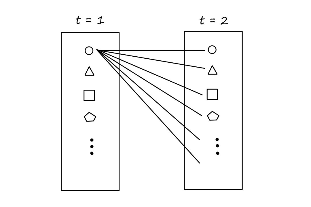
Suppose each shape is a percept. For each percept at `t=1`, there are `|P|` percepts at `t=2` that could be paired with that percept. So `|P|*|P|=|P|^2` total percepts.
Extending that reasoning, for each of the `|P|^2` percept pairs at `t=1,2`, there are `|P|` percepts at `t=3` that could be paired with that percept pair. So `|P|^2*|P|=|P|^3` total percepts.
In general, there are `sum_(t=1)^T |P|^t` possible percept sequences, meaning that the table will have this many entries. An hour's worth of visual input from a single camera can result in at least `10^(600,000,000,000)` percept sequences. Even for chess, there are at least `10^(150)` percept sequences.
So yeah, building such a table is not really possible.
Theoretically though, TABLE-DRIVEN-AGENT does do what we want, which is to implement the agent function. The challenge is to write programs that do this without using a table.
Before the 1970s, people were apparently using huge tables of square roots to do their math. Now there are calculators that run a five-line program implementing Newton's method to calculate square roots.
Can AI do this for general intelligent behavior?
Simple reflex agents
This is the simplest kind of agent. A simple reflex agent selects actions based only on the current percept; it ignores the rest of the percept history. Here's an agent program that implements the agent function for our vacuum:
function REFLEX-VACUUM-AGENT([location, status])
  if status == Dirty then return Clean
  else if location == A then return Move right
  else if location == B then return Move left
Note that since the agent is ignoring the percept history, there are only `4` total possible percepts (not `4^T`) at all times. Square `A` is clean, square `A` is dirty, square `B` is clean, and square `B` is dirty.
Simple reflex behaviors can be modeled as "if-then" statements. If the car in front is braking, then initiate braking. Because of their structure, they are called condition-action rules (or situation-action rules or if-then rules).
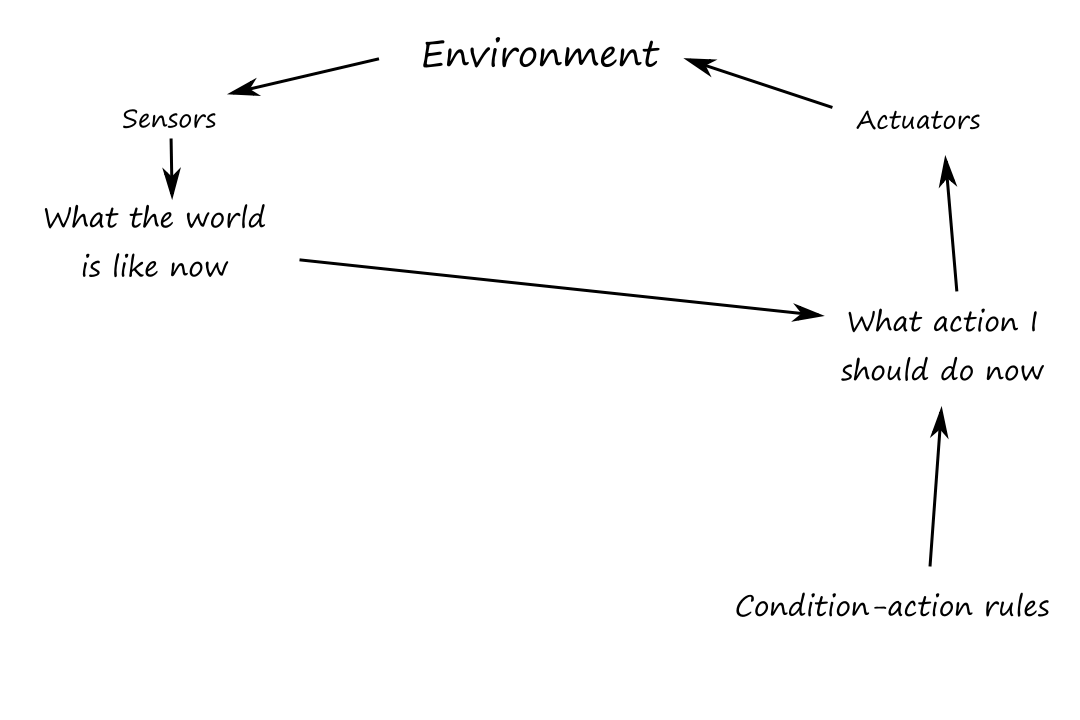
REFLEX-VACUUM-AGENT is specific to the world of just two squares. Here's a more general and flexible way of writing agent programs:
function SIMPLE-REFLEX-AGENT(percept)
  state = INTERPRET-INPUT(percept)
  rule = RULE-MATCH(state, rules)
  action = rule.ACTION
  return action
rules: a set of condition-action rules
This approach involves designing a general-purpose interpreter that can convert a percept to a state. Then we provide the rules for specific states.
While simple reflex agents are, well, simple, they only work well in fully observable environments. The state of the environment has to be easily identifiable, otherwise the wrong rule and action will be applied. For example, it may be hard for the agent to tell if a car is braking or if it's just the taillights that are on.
For our vacuum example, suppose the vacuum didn't have a location sensor. Then it won't know which square it's on. If it starts at square `A` and chooses to move left, it will fail forever (and likewise if it starts at square `B` and chooses to move right).
Infinite loops like these often happen in partially observable environments and can be avoided by having the agent randomize its actions. Randomization can be rational in some multiagent environments, but it is usually not rational in single-agent environments.
Model-based reflex agents
To deal with partial observability, the agent can keep track of the part of the world it can't see now. In order to do this, the agent needs to maintain some sort of internal state that depends on the percept history. For a car changing lanes, the agent needs to keep track of where the other cars are if it can't see them all at once.
In order to update its internal state, the agent needs to know "how the world works". When the agent turns the steering wheel clockwise, the car turns to the right (effect of agent action). When it's raining, the car's camera can get wet (how the world evolves independent of agent's actions). This is a transition model of the world.
The agent also needs to know how to interpret the information it gets from its percepts to understand the current state of the world. When the car in front of the agent brakes, there will be several red regions in the forward-facing camera image. When the camera gets wet, there will be droplet-shaped objects in the image. This knowledge is called a sensor model.
A model-based agent uses the transition model and sensor model to keep track of the state of the world.
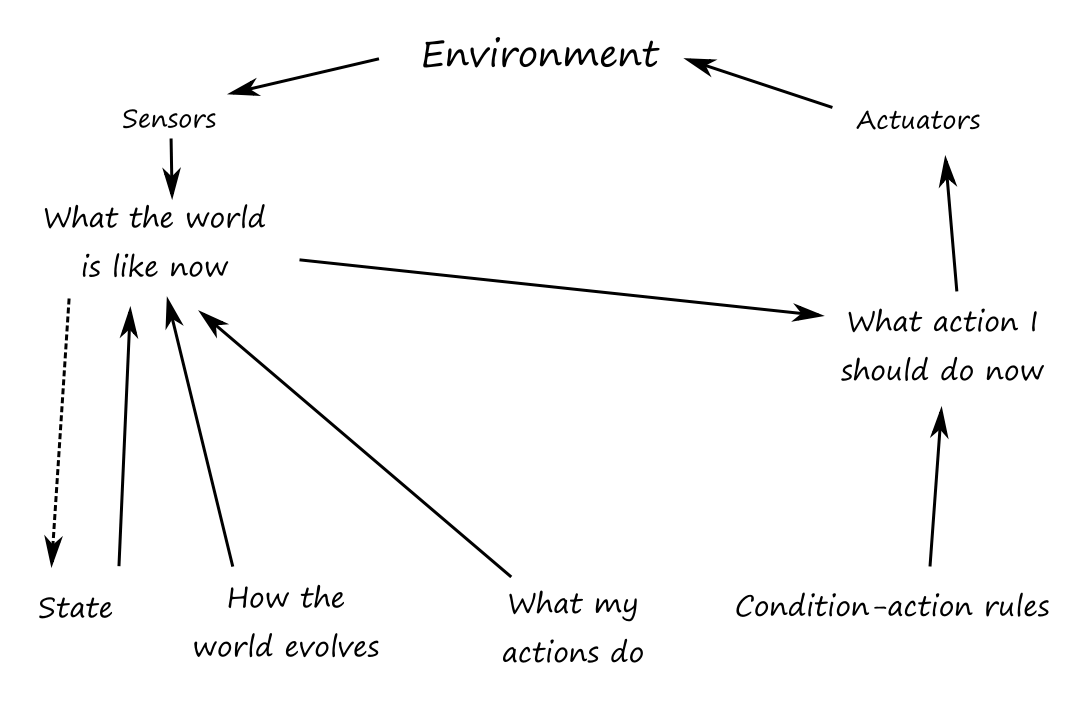
"What the world is like now" is really the agent's best guess.
function MODEL-BASED-REFLEX-AGENT(percept)
  state = UPDATE-STATE(state, action, percept, transition_model, sensor_model)
  rule = RULE-MATCH(state, rules)
  action = rule.ACTION
  return action
state: the agent's current conception of the world state
transition_model: a description of how the next state depends on the current state and action
sensor_model: a description of how the current world state is reflected in the agent's percepts
rules: a set of condition-action rules
action: the agent's most recent action, initially none
Goal-based agents
Sometimes, having information about the current state of the environment is not enough to decide what to do. For example, knowing that there's a fork in the road is not enough; the agent needs to know whether it should go left or right. The correct decision depends on the goal.
Goal-based decision making is different from following condition-action rules because it involves thinking about the future. A reflex agent brakes when it sees brake lights because that's specified in the rules. But a goal-based agent brakes when it sees brake lights because that's how it thinks it will avoid hitting other cars.
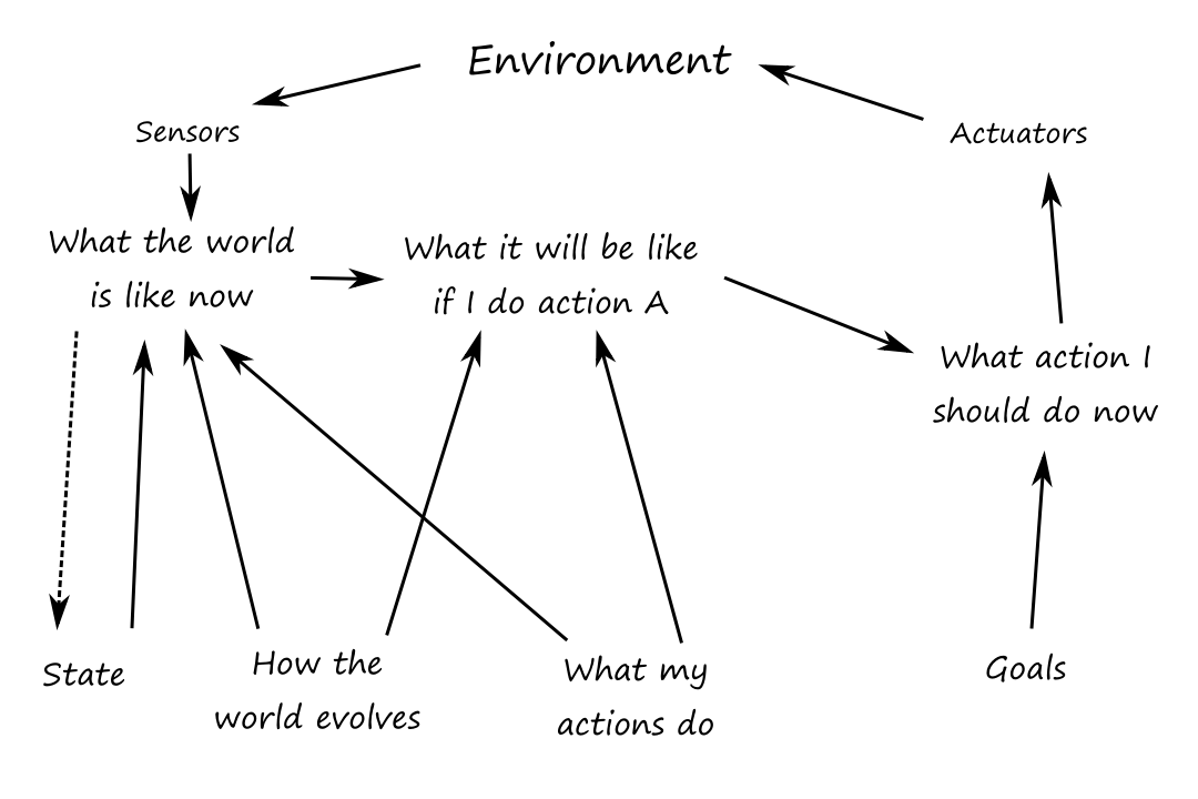
Goal-based agents are also more flexible than reflex agents. If we want a goal-based agent to drive to a different destination, then we just have to update the goal. But if we want a reflex agent to go to a different destination, we have to update all the rules so that they go to the new destination.
Utility-based agents
While achieving the goal is what we want the agent to do, there are many different actions that can be taken to get there. And those different actions can affect how "happy" or "unhappy" the agent will be. This level of "happiness" is referred to as utility.
For example, a quicker/safer/more reliable/cheaper route makes the agent "happier" because it optimizes its performance measure.
A utility function maps environment states to a desirability score. If there are conflicting goals (e.g., speed and safety), the utility function specifies the appropriate tradeoff.
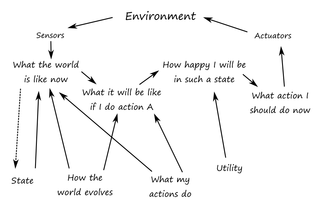
An agent won't know exactly how "happy" it will be if it takes an action. So it's more correct to say that a rational utility-based agent chooses the action that maximizes expected utility (as opposed to just utility).
Learning agents
The preferred way to build agents (model-based, goal-based, utility-based, etc.) is to build them as a learning agent and then teach them.
A learning agent can be divided into four conceptual components: the learning element, the performance element, the critic, and the problem generator. The learning element is responsible for making improvements. The performance element is responsible for selecting actions. The critic provides feedback on how the agent is doing and determines how the performance element should be modified to do better.
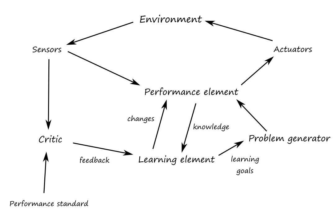
The problem generator is responsible for suggesting actions that will lead to new and informative experiences. This allows the agent to explore some suboptimal actions in the short run that may become much better actions in the long run.
The performance standard can be seen as a mapping from a percept to a reward or penalty. This allows the critic to learn what is good and bad.
The performance standard is a fixed external thing that is not a part of the agent.
For now, we'll assume that the environments are episodic, single agent, fully observable, deterministic, static, discrete, and known.
Problem-Solving Agents
If the agent doesn't know what the correct action to take should be, it should do some problem solving:
- Goal formulation: figure out what the goal is to limit the number of actions that need to be considered
- Problem formulation: describe the states and actions (come up with an abstract model of the world)
- Search: try different sequences of actions to find one (the solution) that achieves the goal
- Execution: just do it
In a fully observable, deterministic, known environment, the solution to any problem is a fixed sequence of actions. For example, traveling from one place to another.
In a partially observable or nondeterministic environment, a solution would be a branching strategy (if/else) that recommends different future actions depending on what percepts the agent sees. For example, the agent might come across a sign that says the road is closed, so it would need a backup plan.
Search problems and solutions
Formally, a search problem can be defined by specifying:
- the state space: the set of possible states that the environment can be in
- the initial state that the agent starts in
- a set of one or more goal states
- the actions available to the agent
- a transition model that describes what each action does
- an action cost function that describes the cost of performing an action
- the cost should reflect the agent's performance measure, such as distance, time, or monetary cost
A sequence of actions forms a path, and a solution is a path from the initial state to a goal state. The cost of a path is the sum of the costs of each action on that path, so an optimal solution is the path with the lowest cost among all solutions. Everything can be represented as a graph where the vertices are the states and the edges are the actions.
Example Problems
Standardized problems
A grid world problem is an array of cells where agents can move from cell to cell and each cell can contain objects. Our little vacuum example is an example of a grid world problem.
- states: there are `8` different states depending on which objects are in which cells
- for each of the two cells, it can contain the vacuum or not and it can contain dirt or not (`2*2*2=8`)
- initial state: any state can be chosen as the initial state
- actions: move left, move right, clean
- transition model: cleaning removes dirt from the agent's cell and move left/right are self-explanatory
- goal states: all the states where every cell is clean
- both cells are clean and the vacuum ends up in the left cell
- both cells are clean and the vacuum ends up in the right cell
- action cost: each action costs `1`
This one's interesting. Donald Knuth conjectured that a sequence of square root, floor, and factorial operations can be applied to the number `4` to reach any positive integer. For example, we can reach `5` by applying eight operations:
`lfloorsqrt(sqrt(sqrt(sqrt(sqrt((4!)!)))))rfloor=5`
- states: positive real numbers
- initial state: `4`
- actions: apply square root, floor, or factorial operation
- transition model: the effect of applying the operations are mathematically defined
- goal state: the desired positive integer
- action cost: each action costs `1`
Real-world problems
A common type of real-world problem is the route-finding problem (finding an optimal path from point A to point B). For example, airline travel:
- states: location and current time
- initial state: our home airport
- actions: take any flight from the current location
- transition model: the flight's destination will become our new current location and the flight's arrival time will become our new current time
- goal state: our destination
- the goal can also be "arrive at the destination on a nonstop flight"
- action cost: combination of monetary cost, waiting time, flight time, seat quality, time of day, type of airplane, frequent-flyer reward points, etc.
Touring problems is an extension of the route-finding problem where multiple locations must be visited instead of just one destination. The traveling salesperson problem is a popular example.
Search Algorithms
Search problems can be represented as a search tree, where a node represents a state and the edges represent the actions. For Knuth's conjecture:
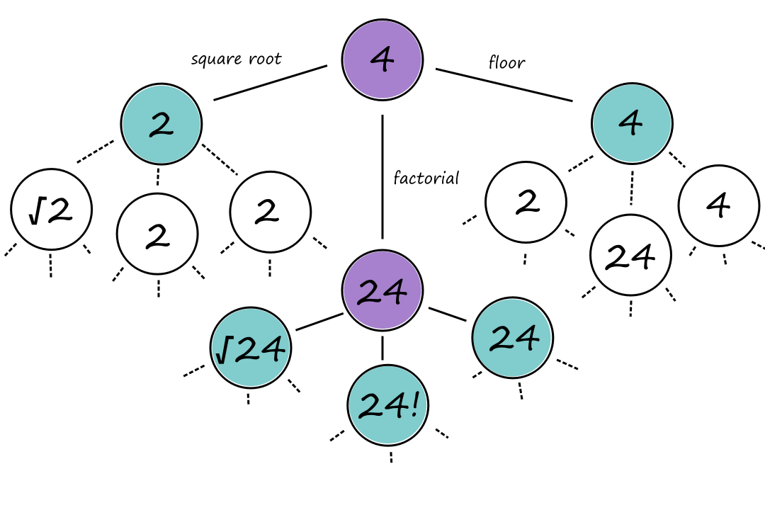
The purple nodes are nodes that have been expanded. The green nodes are nodes that are on the frontier, i.e., they have not been expanded yet.
When we're at a node, we can expand the node to consider the available states that are possible (generate nodes). The nodes that have not been expanded yet make up the frontier of the search tree.
Best-first search
So how do we decide which path to take? A good general approach is to perform best-first search. In this type of search, we define an evaluation function, which, in a sense, is a measure of how close we are to reaching the goal state. When we apply the evaluation function to each frontier node, the node with the minimum value of the evaluation function should be the next node to go to.
One example of an evaluation function for Knuth's conjecture could be
`f(n) = abs(n-G)`
where `n` is the current node and `G` is the goal. This evaluation function is measuring the distance between where we are and where we want to be, so it makes sense to choose the node that minimizes this distance. Unfortunately, this isn't a very helpful evaluation function to use because it would tell us to keep applying the floor operation.
Search data structures
We can implement a node by storing:
- state: the state of the node
- parent: the node that generated this node
- action: the action that was applied to the parent to generate this node
- path-cost: the total cost of the path from the initial state to this node
We can store the frontier using a queue. A queue is good because it provides us with the operations to check if a frontier is empty, take the top node from the frontier, look at the top node of the frontier, and add a node to the frontier.
function BEST-FIRST-SEARCH(problem, f)
  node = NODE(STATE = problem.INITIAL)
  frontier = priority queue ordered by f
  reached = a lookup table
  while not IS-EMPTY(frontier) do
    node = POP(frontier)
    if problem.IS-GOAL(node.STATE) then return node
    for each child in EXPAND(problem, node) do
      s = child.STATE
      if s is not in reached or child.PATH-COST < reached[s].PATH-COST then
        reached[s] = child
        add child to frontier
  return failure
function EXPAND(problem, node)
  s = node.STATE
  for each action in problem.ACTIONS do
    s' = problem.RESULT(s, action)
    cost = node.PATH-COST + problem.ACTION-COST(s, action, s')
    yield NODE(STATE = s', PARENT = node, ACTION = action, PATH-COST = cost)
Redundant paths
As we traversing the tree, it's possible to get stuck in a cycle (loopy path), i.e., go around in circles through repeated states. Here's an example of a cycle:
`4 ubrace(rarr)_(text(factorial)) 24 ubrace(rarr)_(text(square root)) 4.9 ubrace(rarr)_(text(floor)) 4`
A cycle is a type of redundant path, which is a path that has more steps than necessary. Here's an example of a redundant path:
`4 ubrace(rarr)_(text(floor)) 4 ubrace(rarr)_(text(square root)) 2`
(This is redundant because we could've just gone to `2` directly without needing the first floor operation.)
There are three ways to handle the possibility of running into redundant paths. The preferred way is to keep track of all the states we've been to. That way, if we see it again, then we know not to go that way. (The best-first search pseudocode does this.)
The bad part about doing this is that there might not be enough memory to keep track of all this info. So we can check for cycles instead of redundant paths. We can do this by following the chain of parent pointers ("going up the tree") to see if the state at the end has appeared earlier in the path.
Or we can choose to not even worry about choosing redundant paths if it's rare or impossible to have them. From this point on, we'll use graph search for search algorithms that check redundant paths and tree-like search for ones that don't.
Uninformed Search Strategies
The uninformed means that as the agent is performing the search algorithm, it doesn't know how close the current state is to the goal.
Breadth-first search
In breadth-first search, all the nodes on the same level are expanded first before going further down any paths. This is generally a good strategy to consider when all the actions have the same cost.
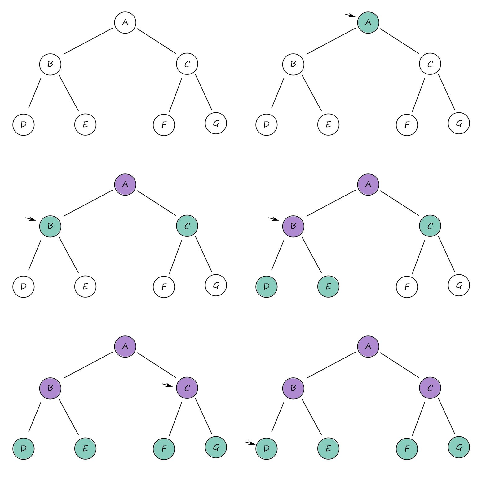
Breadth-first search can be implemented as a call to BEST-FIRST-SEARCH where the evaluation function is the depth of the node, i.e., the number of actions it takes to reach the node.
There are several optimizations we can take advantage of when using breadth-first search. Using a first-in-first-out (FIFO) queue is faster than using a priority queue because the nodes that get added to a FIFO queue will already be in the correct order (so there's no need to perform a sort, which we would need to do with a priority queue).
Best-first search waits until the node is popped off the queue before checking if it's a solution (late goal test). But with breadth-first search, we can check if a node is a solution as soon as it's generated (early goal test). This is because traversing breadth first explores all the possible paths above the generated node, guaranteeing that we've found the shortest path to it. (Think about it like this: because we're traversing breadth first, we can't say, "Would we have found a shorter way here if we had gone on that path instead?" because we already checked that path.)
Because of this, breadth-first search is cost-optimal for problems where all actions have the same cost.
function BREADTH-FIRST-SEARCH(problem)
  node = NODE(problem.INITIAL)
  if problem.IS-GOAL(node.STATE) then return node
  frontier = a FIFO queue
  reached = {problem.INITIAL}
  while not IS-EMPTY(frontier) do
    node = POP(frontier)
    for each child in EXPAND(problem, node) do
      s = child.STATE
      if problem.IS-GOAL(s) then return child
      if s is not in reached then
        add s to reached
        add child to frontier
  return failure
Let `d` represent the depth of the search tree. Suppose each node generates `b` child nodes.
The root node generates `b` nodes. Each of those `b` nodes generates `b` nodes (total `b^2` nodes). And each of the `b^2` nodes generates `b` nodes (total `b^3` nodes). So the total number of nodes generated is
`1+b+b^2+b^3+...+b^d=O(b^d)`
Time and space complexity are exponential, which is bad. (All the generated nodes have to remain in memory.)
Dijkstra's algorithm or uniform-cost search
If actions have different costs, then uniform-cost search is a better consideration. The main idea behind this is that the least-cost paths are explored first. (I go into more step-by-step detail about how Dijkstra's algorithm works in my Computer Networking resource.)
Uniform-cost search will always find the optimal solution, but the main problem with it is that it's inefficient. It will expand a lot of nodes.
Uniform-cost search can be implemented as a call to BEST-FIRST-SEARCH where the evaluation function is the cost of the path from the root to the current node.
The worst-case time and space complexity is `O(b^(1+lfloorC^**//epsilonrfloor))` where `C^**` is the cost of the optimal solution and `epsilon` is a lower bound on the cost of all actions.
Since costs are positive (`gt 0`), going down one path by one node may be "deeper" than going down another path by one node, so we can't use the same `d` notation for depth. So `C^(**)/epsilon` is an upper bound on how deep the solution is, i.e., the max number of actions that are taken to reach the solution.
Depth-first search
In depth-first search, the deepest node in the frontier is expanded first. Basically, one path at a time is picked and followed until it ends. So if a goal state is found, then that path is chosen as the solution. This also means that the path chosen may not be the cheapest path available. (What if we had gone down that path instead?)
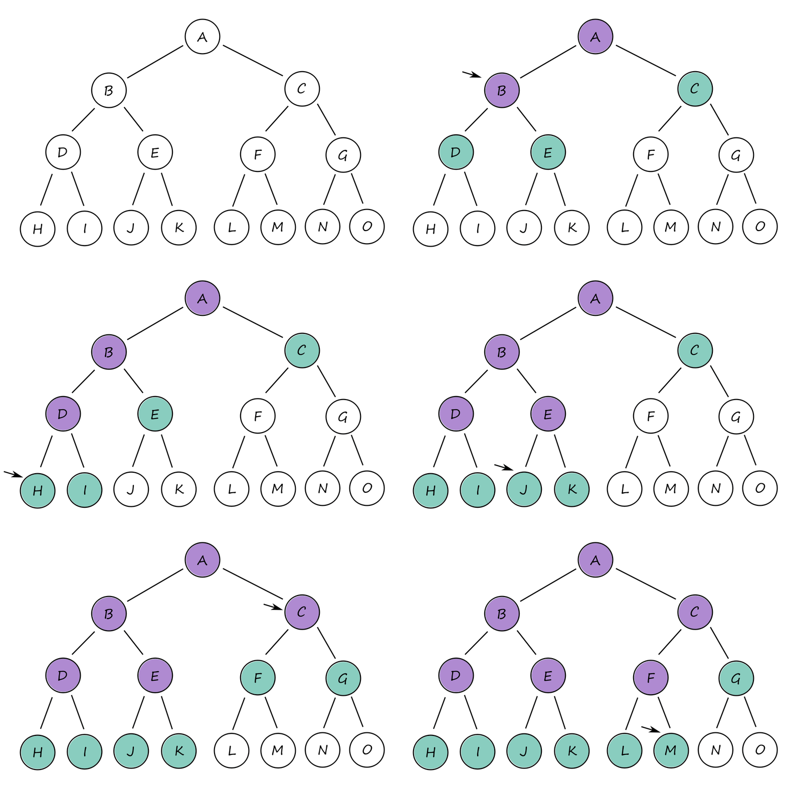
So why should this algorithm even be considered? It's because depth-first search doesn't require a lot of memory. There's no need for a reached table and the frontier is very small.
The frontier of breadth-first search can be thought of as the surface of an expanding sphere while the frontier of depth-first search can be thought of as the radius of that sphere.
The memory complexity is `O(bm)` where `b` is the branching factor (number of nodes on a branch) and `m` is the maximum depth of the tree. Whenever we expand a node, we add `b` generated children to the frontier. Then we move to one of the children, generate its `b` children, and add them to the frontier. And so on until the bottom. This happens `m` times. So at the bottom, there are `m` groups of `b` children in the frontier.
Depth-first search can be implemented as a call to BEST-FIRST-SEARCH where the evaluation function is the negative of the depth.
Depth-limited and iterative deepening search
Another problem with depth-first search is that it can keep going down one path infinitely. To prevent this, we can decide to stop going down a path once we reach a certain point. This is depth-limited search.
The time complexity is `O(b^l)` and the space complexity is `O(bl)` for the same reasons as depth-first search.
But how far is too far? If we stop too early, we may not find a solution and if we choose to stop very late, it will take a long time. Iterative deepening search keeps trying different stopping points until a solution is found or until no solution is found (if this is the case, then we have gone deep enough to the point where all paths can be fully explored).
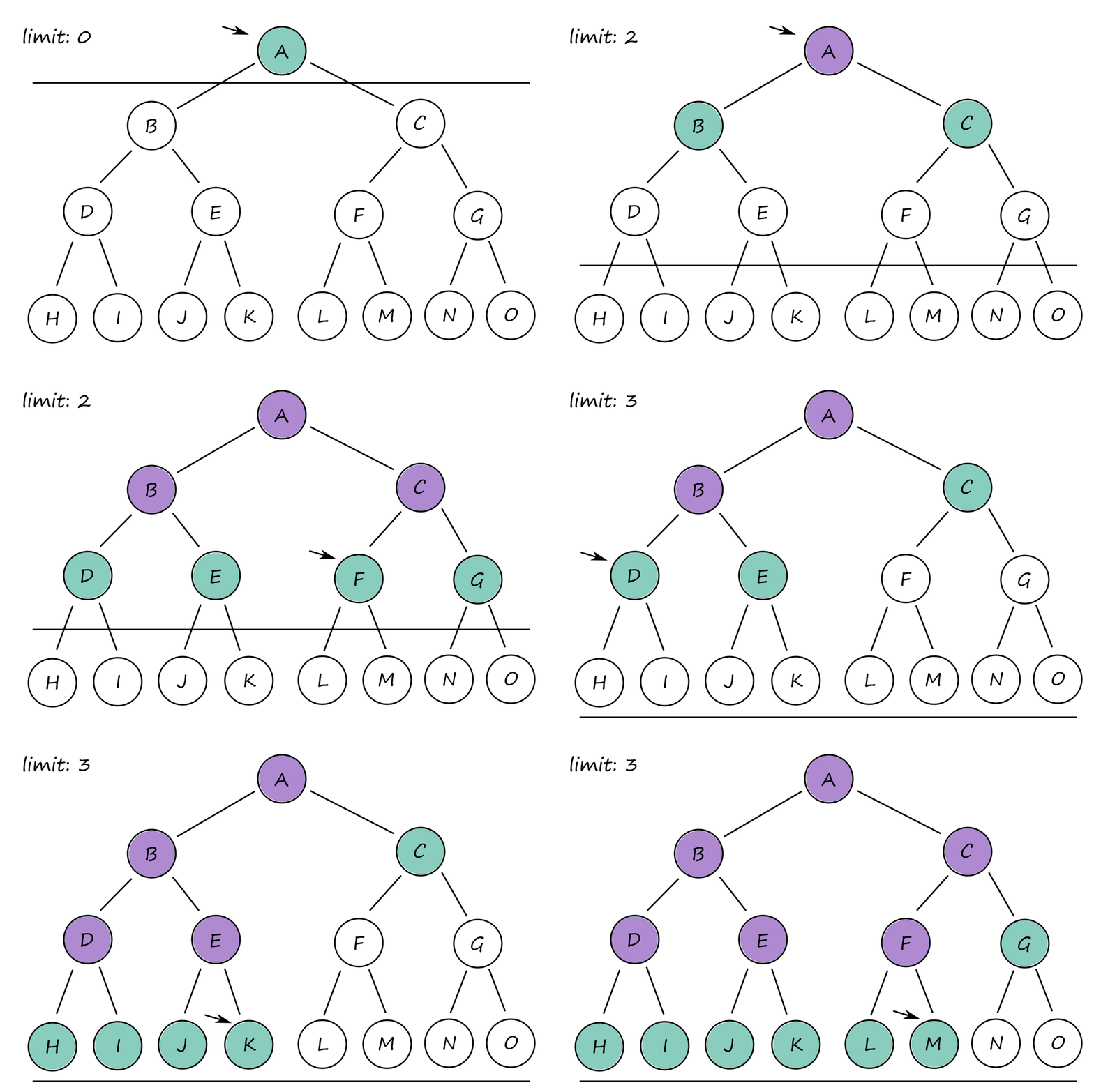
It may seem a bit repetitive (or wasteful) to keep generating the top-level nodes. For example, `B` and `C` are generated `3` times at limits `1`, `2`, and `3`. However, this isn't really that big of an issue since the majority of the nodes are at the bottom, and those are only generated a few times compared to the top-level nodes.
In general, the nodes at the bottom level are generated once, those on the next-to-bottom level are generated twice, ..., and the children of the root are generated `d` times. So the total number of nodes generated is
`(d)b^1+(d-1)b^2+(d-2)b^3+...+b^d=O(b^d)`
So the time complexity is `O(b^d)` when there's a solution (and `O(b^m)` when there isn't).
The memory complexity is `O(bd)` when there is a solution and `O(bm)` when there isn't (for finite state spaces).
function DEPTH-LIMITED-SEARCH(problem, l)
  frontier = a LIFO queue
  result = failure
  while not IS-EMPTY(frontier) do
    node = POP(frontier)
    if problem.IS-GOAL(node.STATE) then return node
    if DEPTH(node) > l then
      result = cutoff
    else if not IS-CYCLE(node) do
      for each child in EXPAND(problem, node) do
        add child to frontier
  return result
function ITERATIVE-DEEPENING-SEARCH(problem)
  for depth = 0 to infinity do
    result = DEPTH-LIMITED-SEARCH(problem, depth)
    if result != cutoff then return result
cutoff is a string used to denote that there might be a solution at a deeper level than `l`.
Iterative deepening is the preferred uninformed search method when the search state space is larger than can fit in memory and the depth of the solution is not known.
Bidirectional search
So far, all the algorithms started at the initial state and moved towards a goal state. But what we can also do is start from the initial state and the goal state(s) and hope that we meet somewhere in the middle. This is bidirectional search.
We need to keep track of two frontiers and two tables of reached states. There is a solution when the two frontiers meet.
Even though we have to keep track of two frontiers, each frontier is only half the size of the whole tree. So the time and space complexity is `O(b^(d//2))`, which is less than `O(b^d)`.
function BIBF-SEARCH(problem_F, f_F, problem_B, f_B)
  node_F = NODE(problem_F.INITIAL)
  node_B = NODE(problem_B.INITIAL)
  frontier_F = a priority queue ordered by f_F
  frontier_B = a priority queue ordered by f_B
  reached_F = a lookup table
  reached_B = a lookup table
  solution = failure
  while not TERMINATED(solution, frontier_F, frontier_B) do
    if f_F(TOP(frontier_F)) < f_B(TOP(frontier_B)) then
      solution = PROCEED(F, problem_F, frontier_F, reached_F, reached_B, solution)
    else solution = PROCEED(B, problem_B, frontier_B, reached_B, reached_F, solution)
  return solution
function PROCEED(dir, problem, frontier, reached, reached_2, solution)
  node = POP(frontier)
  for each child in EXPAND(problem, node) do
    s = child.STATE
    if s not in reached or PATH-COST(child) < PATH-COST(reached[s]) then
        reached[s] = child
        add child to frontier
        if s is in reached_2 then
          solution_2 = JOIN-NODES(dir, child, reached_2[s])
          if PATH-COST(solution_2) < PATH-COST(solution) then
            solution = solution_2
  return solution
TERMINATED determines when to stop looking for solutions and JOIN-NODES joins the two paths.
Comparing uninformed search algorithms
An algorithm is complete if either a solution is guaranteed to be found if it exists or a failure is reported when it doesn't exist.
| Criterion | Breadth-First | Uniform-Cost | Depth-First | Depth-Limited | Iterative Deepening | Bidirectional |
|---|---|---|---|---|---|---|
| Complete? | Yes* | Yes*† | No | No | Yes* | Yes*§ |
| Optimal cost? | Yes‡ | Yes | No | No | Yes‡ | Yes‡§ |
| Time | `O(b^d)` | `O(b^(1+lfloorC^**//epsilonrfloor))` | `O(b^m)` | `O(b^l)` | `O(b^d)` | `O(b^(d//2))` |
| Space | `O(b^d)` | `O(b^(1+lfloorC^**//epsilonrfloor))` | `O(bm)` | `O(bl)` | `O(bd)` | `O(b^(d//2))` |
`b` is the branching factor. `m` is the maximum depth of the search tree. `d` is the depth of the shallowest solution, or is `m` when there is no solution. `l` is the depth limit.
*if `b` is finite
†if all action costs are `ge epsilon gt 0`
‡if all action costs are identical
§if both directions are breadth-first or uniform-cost
Informed (Heuristic) Search Strategies
Informed means that information is provided about how close the current state is to a goal state.
The information is referred to as "hints", which are given by a heuristic function, denoted as `h(n)`.
`h(n)=` estimated cost of the cheapest path from the state at node `n` to a goal state
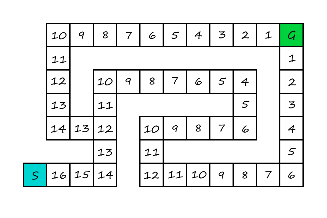
For the next few algorithms, we'll be using this maze, where the goal is to find the shortest path from `S` to `G`. The number in each square is the number of squares it is away from the goal (ignoring walls). That is the heuristic we'll be using.
Greedy best-first search
If we know how close each node is to a goal, then it seems to makes sense to choose the node that seems closest to the goal.
We expand first the node with the lowest `h(n)` value.
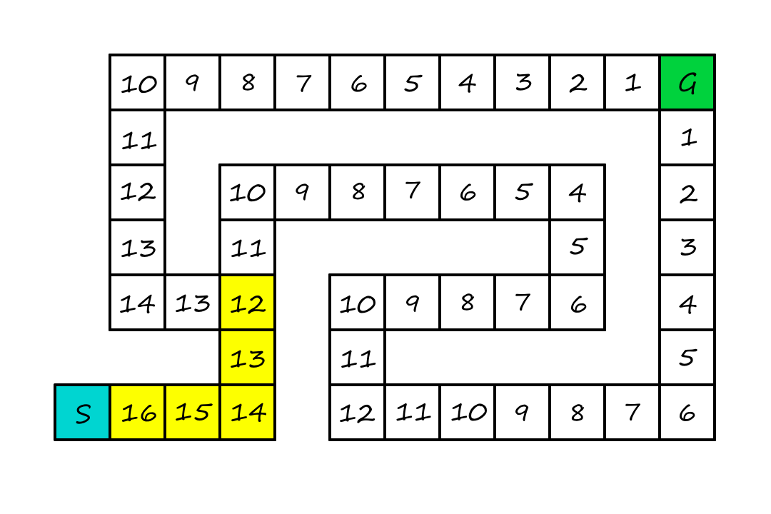
Since we're being greedy, we'll move to the square that looks like it's `11` squares away from the goal instead of the square that looks like it's `13` squares away from the goal.
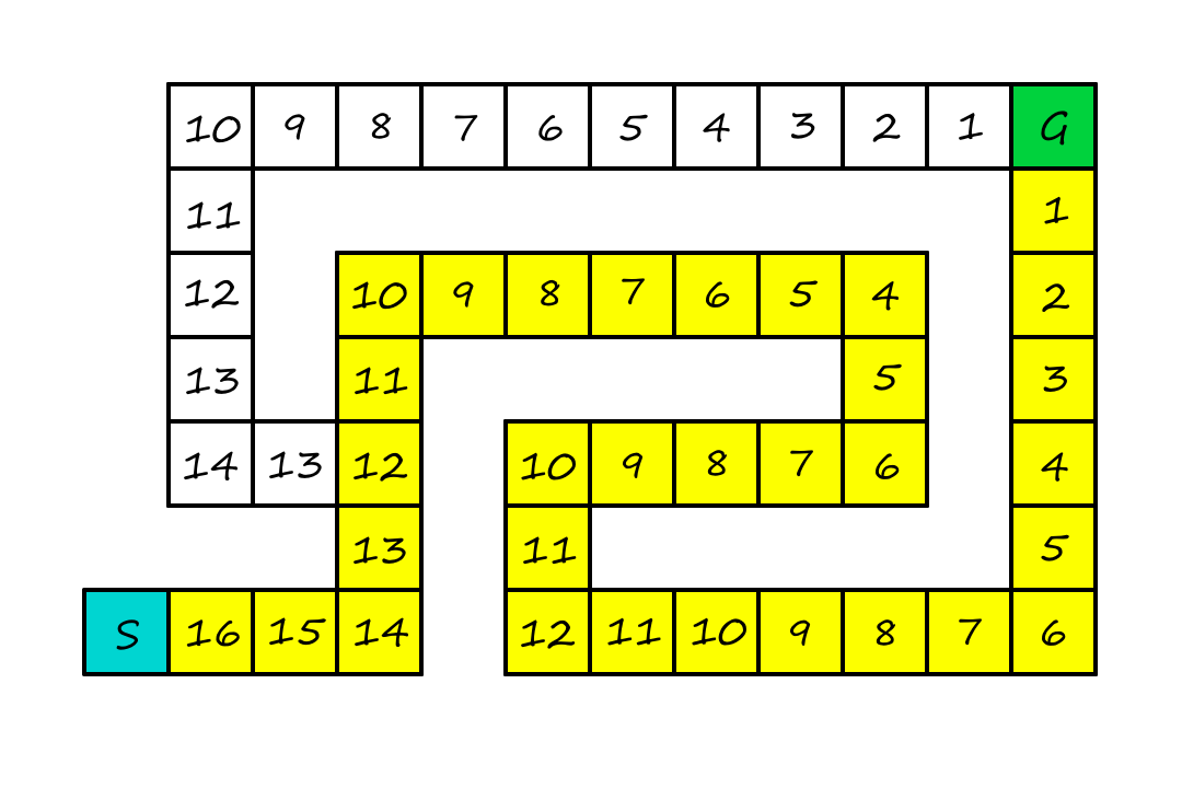
Now obviously, this is not the optimal path. But being greedy is not always a good thing.
A* search
The reason greedy best-first search failed is because it didn't take into consideration the cost of going to each node -- it only looked at how far away each node was to the destination. Intuitively, if it takes a long time to get to a destination that is close to your goal, is it really worth going to that destination? A* search looks at both the cost to get to each node and the estimated cost from each node to the destination.
A* search can be implemented as a call to BEST-FIRST-SEARCH where the evaluation function is `g(n)+h(n)`. `g(n)` is the cost from the initial state to node `n`, and `h(n)` is the estimated cost of the shortest path from `n` to a goal state.
`f(n)=` estimated cost of the best path that continues from `n` to a goal
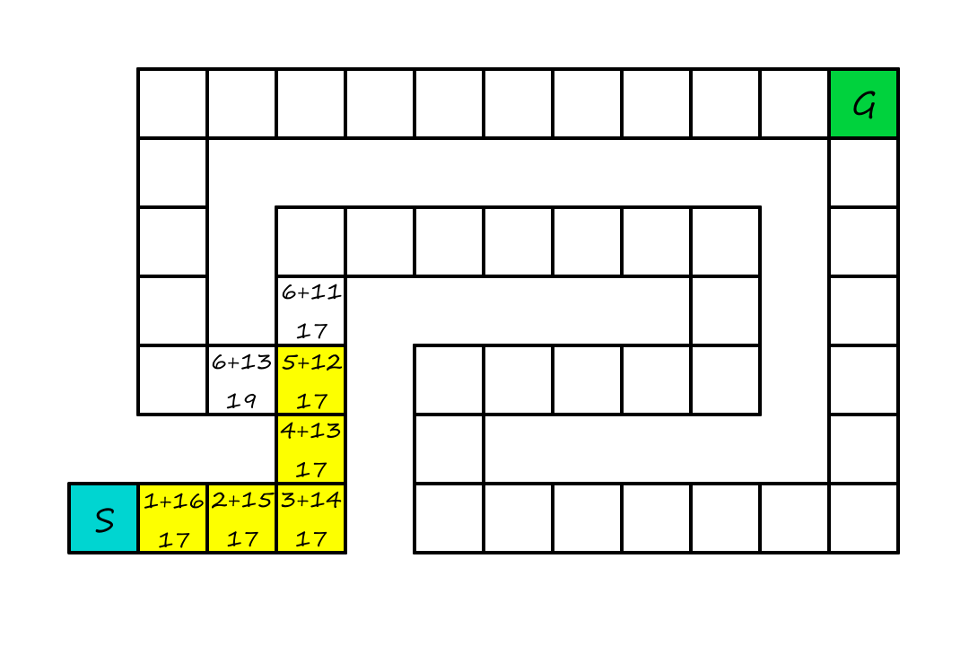
Now, the numbers in each square represent the cost of going to that square plus the estimated distance to the goal, i.e., the number of squares it is away from the goal (ignoring walls).
Just like in greedy search, we'll be going up again. But don't worry, things will be different this time.
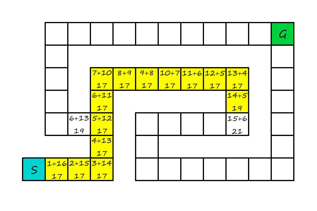
At this point, we see that it's no longer worth continuing on this path because there is a cheaper option (`19`) at the fork. So we'll start going that way instead.
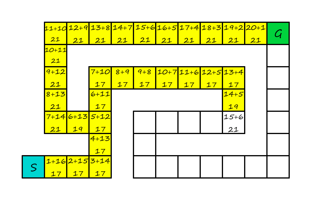
Even though we wasted some time going down the longer path, we still found the optimal solution.
Whether A* is cost-optimal depends on the heuristic. If the heuristic is admissible, then A* is cost-optimal. Admissible means that the heuristic never overestimates the cost to reach a goal, i.e., the estimated cost to reach the goal is `le` the actual cost to reach the goal. Admissible heuristics are referred to as being optimistic.
We can show A* is cost-optimal with an admissible heuristic by using a proof by contradiction.
Let `C^**` be the cost of the optimal path. Suppose for the sake of contradiction that the algorithm returns a path with cost `C gt C^**`. This means that there is some node `n` that is on the optimal path and is unexpanded (if we had expanded it, we would've found the optimal path and returned `C^**` instead).
Let `g^(ast)(n)` be the cost of the optimal path from the start to `n`, and let `h^(ast)(n)` be the cost of the optimal path from `n` to the nearest goal.
`f(n) gt C^**` (otherwise `n` would've been expanded)
`f(n) = g(n)+h(n)` (by definition)
`f(n) = g^(ast)(n)+h(n)` (because `n` is on the optimal path)
`f(n) le g^(ast)(n)+h^(ast)(n)` (because of admissibility, `h(n) le h^(ast)(n)`)
`f(n) le C^**` (by definition, `C^(ast)=g^(ast)(n)+h^(ast)(n)`)
The first and last lines form a contradiction. So it must be the case that the algorithm returns a path with cost `C le C^**`, i.e., A* is cost-optimal.
A heuristic can also be consistent, which is slightly stronger than being admissible (so every consistent heuristic is admissible). A heuristic `h(n)` is consistent if, for every node `n` and every successor `n'` of `n` generated by action `a`,
`h(n) le c(n,a,n') + h'(n)`
What this is saying is that the estimated cost to the goal from our current position should be less than (or equal to) the cost of going to another location plus the estimated cost of going to the goal from that location. In other words, adding a stop should make the trip longer unless that stop is on the way to the destination.
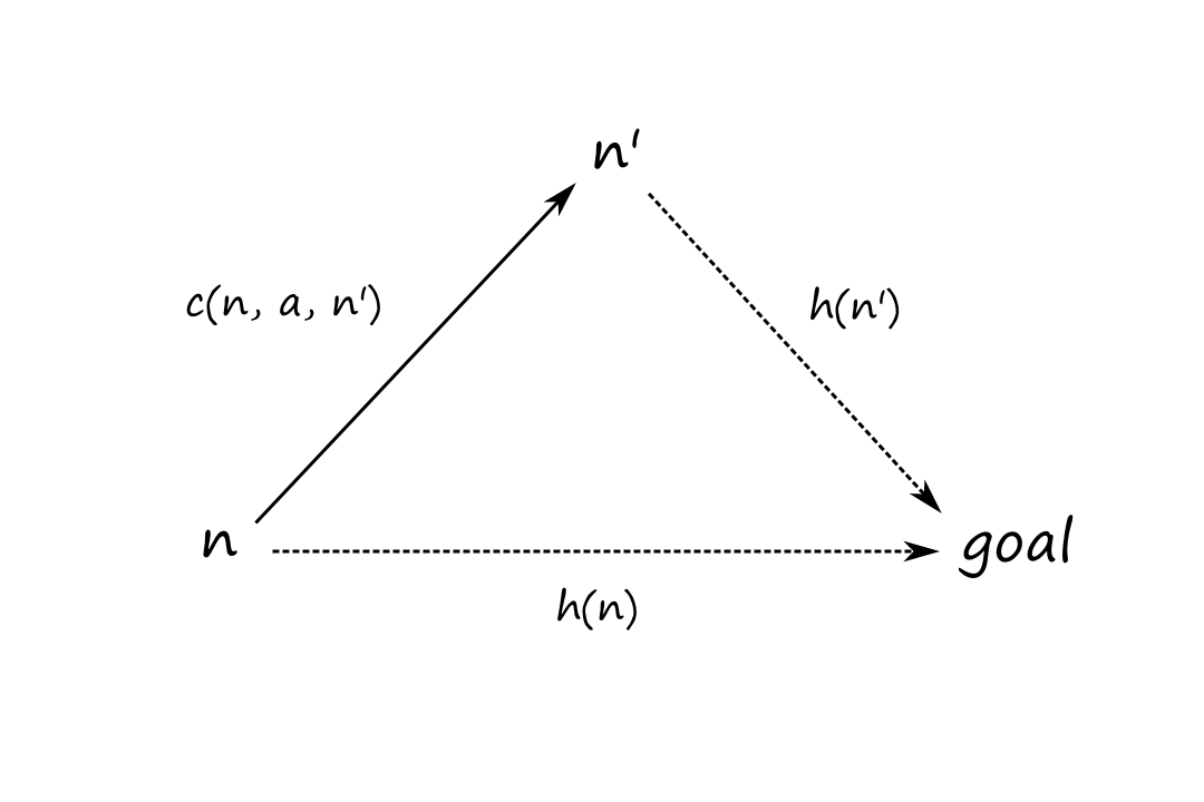
Consistency is a form of the triangle inequality, which says that a side of a triangle can't be longer than the sum of the other two sides.
Here's an example of how things can be not optimal if the heuristic is not admissible/consistent.
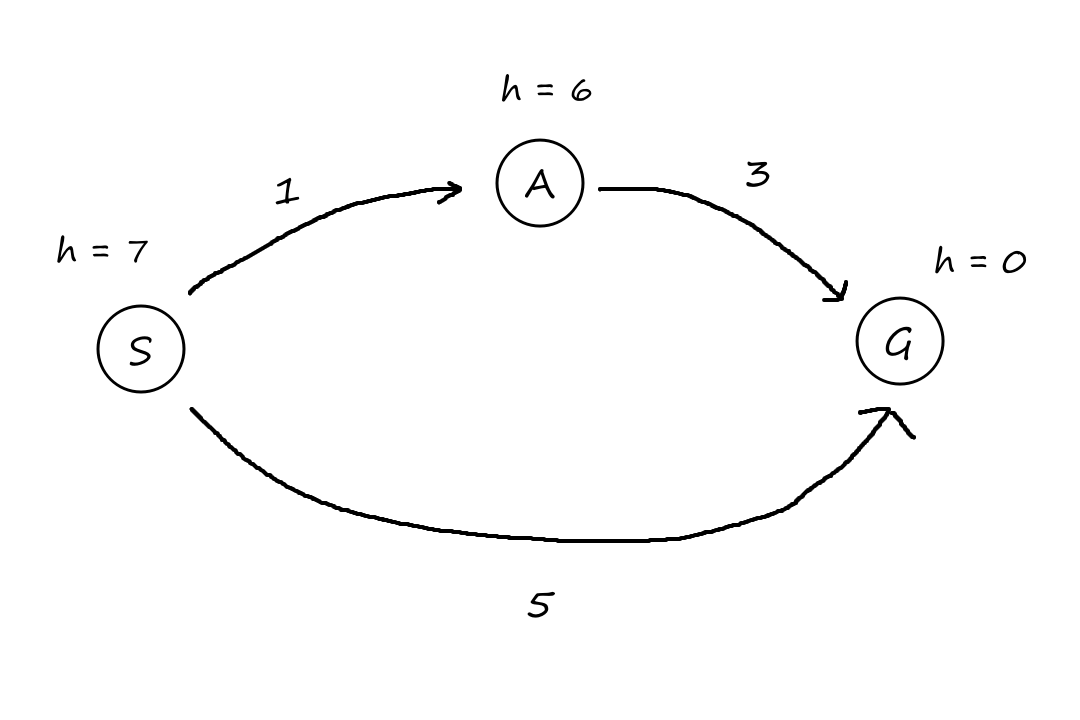
When we're starting at `S`, we can either choose to go to `A` or to `G` directly. Since the estimated cost of `A rarr G` is `6`, it looks more expensive to go to `A` first, so we go to `G` directly instead (`f(A)=1+6=7 gt f(G)=5+0=5`).
However, `S rarr G` is not the optimal path! `S rarr G` costs `5` while `S rarr A rarr G` costs `4`.
This happened because we overestimated the distance from `A` to `G`.
As we go down a path, the `g` costs should be increasing because action costs are always positive. For our maze example, the closer we get to `G`, the farther we get from `S`. So the distance from `S` to our current position should always be increasing as we keep moving. The `g` costs are (strictly) monotonic.
So does this mean that `f=g+h` will also monotonically increase? As we move from `n` to `n'`, the cost goes from `g(n)+h(n)` to `g(n)+c(n,a,n')+h(n')`. Canceling out the `g(n)`, we see that the path's cost will be monotonically increasing if and only if `h(n) le c(n,a,n')+h(n')`, i.e., if and only if the heuristic is consistent.
So if A* search is using a consistent heuristic, then:
- all nodes that can be reached from the initial state and satisfy `f(n) lt C^(**)` will be expanded (surely expanded nodes)
- this is because `f` is monotonically increasing
- if `f` wasn't monotonically increasing, then if we expand a node, there could be a successor with a lower `f` value, which means there was a better path to get to that successor that we missed (i.e., a node with `f(n) lt C^(**)` wasn't expanded)
- but A* works by picking the nodes with the lowest `f`-values to expand, so we couldn't have missed that better path -- there's a contradiction
- if `f` wasn't monotonically increasing, then if we expand a node, there could be a successor with a lower `f` value, which means there was a better path to get to that successor that we missed (i.e., a node with `f(n) lt C^(**)` wasn't expanded)
- this means that all potential paths with lower costs are explored (ensuring cost-optimality and completeness I think)
- this is because `f` is monotonically increasing
- some nodes where `f(n)=C^(**)` might be expanded
- nodes where `f(n) gt C^(**)` are not expanded
These three things lead to A* with a consistent heuristic being referred to as optimally efficient.
Satisficing search: Inadmissible heuristics and weighted A*
Even though A* is complete, cost-optimal, and optimally efficient, the one big problem with A* is that it expands a lot of nodes, which takes time and uses up space. We can expand fewer nodes by using an inadmissible heuristic, which may overestimate the estimated cost to the goal. Intuitively, if the estimated costs of some of the nodes are higher, then there will be fewer nodes that look favorable to expand. Of course, if we overestimate, then there's a chance we might miss an optimal path, but this is the price to pay for expanding fewer nodes. We might end up with suboptimal, but "good enough" solutions (satisficing solutions).
Inadmissible heuristics are potentially more accurate. Consider a heuristic that uses a straight-line distance to estimate the distance of a road between two cities. The path between two cities is almost never a straight line, so the length of the actual path will be greater than the length of the straight line. Meaning that overestimating the straight-line distance by a little bit will make it closer to the length of the actual path.
We don't actually need an inadmissible heuristic to take advantage of the faster speed and lower memory usage. We can simulate an inadmissible heuristic by adding some weight to the heuristic.
`f(n)=g(n)+W*h(n)`
for some `W gt 1`
This is weighted A* search.
In general, if the optimal cost is `C^(**)`, weighted A* search will find a solution that costs between `C^(**)` and `W*C^(**)`. In practice, it's usually much closer to `C^(**)` than to `W*C^(**)`.
Weighted A* can be seen as a generalization of some of the other search algorithms:
| A* search | `g(n)+h(n)` | `W=1` |
| Uniform-cost search | `g(n)` | `W=0` |
| Greedy best-first search | `h(n)` | `W=oo` |
| Weighted A* search | `g(n)+W*h(n)` | `1 lt W lt oo` |
Memory-bounded search
Beam search keeps only `k` nodes with the best `f`-scores in the frontier. This means that we may be excluding cost-optimal paths (and even solutions), but it's the price to pay to limit the number of expanded nodes. Though for many problems, it can find near-optimal solutions.
Iterative-deepening A* search (IDA*) is a commonly used algorithm for problems with limited memory. Where iterative deepening search uses depth as the cutoff, iterative-deepening A* search uses `f`-cost as the cutoff. Specifically, the cutoff value is the smallest `f`-cost of any node that exceeded the cutoff on the previous iteration.
Once the cutoff is reached, IDA* starts over from the beginning. Recursive best-first search (RBFS) also uses `f`-values to determine how far down a path it should go, but once the cutoff is reached, it steps back and takes another path (the one with the second-lowest `f`-value) instead of starting over.
function RECURSIVE-BEST-FIRST-SEARCH(problem)
  solution, fvalue = RBFS(problem, NODE(problem.INITIAL), infinity)
  return solution
function RBFS(problem, node, f_limit)
  if problem.IS-GOAL(node.STATE) then return node
  successors = LIST(EXPAND(node))
  if successors is empty then return failure, infinity
  for each s in successors do
    s.f = max(s.PATH-COST + h(s), node.f)
  while true do
    best = the node in successors with the lowest f-value
    if best.f > f_limit then return failure, best.f
    alternative = the second lowest f-value among successors
    result, best.f = RBFS(problem, best, min(f_limit, alternative))
    if result != failure then return result, best_f
Bidirectional heuristic search
Bidirectional search is sometimes more efficient than unidirectional search, sometimes not. If we're using a very good heuristic, then A* search will perform well and adding bidirectional search won't add any more value. If we're using an average heuristic, bidirectional search tends to expand fewer nodes. If we're using a bad heuristic, then both directional and unidirectional search will be equally bad.
If we want to use bidrectional search with a heuristic, it turns out that using `f(n)=g(n)+h(n)` as the evaluation function doesn't guarantee that we'll find an optimal-cost solution. Instead, we need two different evaluation functions, one for each direction:
`f_F(n)=g_F(n)+h_F(n)` for going in the forward direction (initial state to goal)
`f_B(n)=g_B(n)+h_B(n)` for going in the backward direction (goal to initial state)
This is a front-to-end search.
Suppose the heuristic is admissible. Let's say that we're in the middle of running the algorithm and the forward direction is currently at node `j` and the backward direction is currently at node `t`. We can define a lower bound on the cost of a solution path `text(initial) rarr ... rarr j rarr ... rarr t rarr ... rarr text(goal)` as
`lb(j,t)=max(g_F(j)+g_B(t), f_F(j), f_B(t))`
The optimal cost must be at least the cost of `text(initial) rarr ... rarr j` plus the cost of `text(goal) rarr ... rarr t`.
Since we're using an admissible heuristic, the estimated costs are underestimated. So the optimal cost must also be at least the cost of `text(initial) rarr ... rarr j` plus the estimated cost of `j rarr ... rarr text(goal)`. The same reasoning applies for `f_B(t)`.
So for any pair of nodes `j,t` with `lb(j,t) lt C^(**)`, either `j` or `t` must be expanded because the path that goes through them is a potential optimal solution. The problem is that we don't know for sure which node is better to expand -- that part's just up to luck.
Either way, this lower bound gives us an idea for an evaluation function we could use:
`f_2(n)=max(2g(n), g(n)+h(n))`
This function guarantees that a node with `g(n) gt C^(**)/2` will never be expanded. If `g(n) gt C^(**)/2`, then `2g(n) gt C^(**)`.
- if `2g(n) ge g(n)+h(n)`, then `f_2(n)=2g(n) gt C^(**)`
- if `2g(n) lt g(n)+h(n)`, then `f_2(n)=g(n)+h(n) gt 2g(n) gt C^(**)`
So `f_2(n) gt C^(**)` for nodes with `g(n) gt C^(**)/2`. But nodes on optimal paths will have `f_2(n) le C^(**)`, so those will be expanded first.
Here's another example of greedy search, A* search, and RBFS from the textbook.
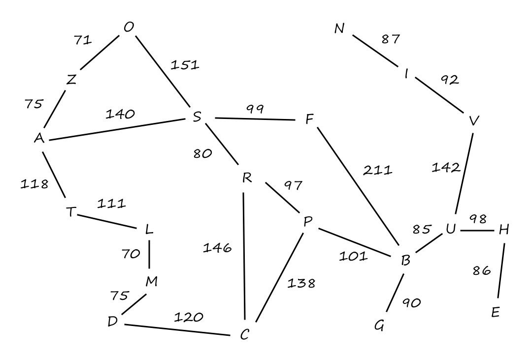
The map uses straight lines, but it's just a drawing. The roads aren't necessarily straight lines.
| City | Straight-line distance to B |
|---|---|
| A | 366 |
| B | 0 |
| C | 160 |
| D | 242 |
| E | 161 |
| F | 176 |
| G | 77 |
| H | 151 |
| I | 226 |
| L | 244 |
| City | Straight-line distance to B |
|---|---|
| M | 241 |
| N | 234 |
| O | 380 |
| P | 100 |
| R | 193 |
| S | 253 |
| T | 329 |
| U | 80 |
| V | 199 |
| Z | 374 |
Greedy best-first search
Let's say we're starting at `A` and we want to go to `B`. If we use the straight-line distance heuristic, then we get the path `A ubrace(rarr)_(140) S ubrace(rarr)_(99) F ubrace(rarr)_(211) B`.
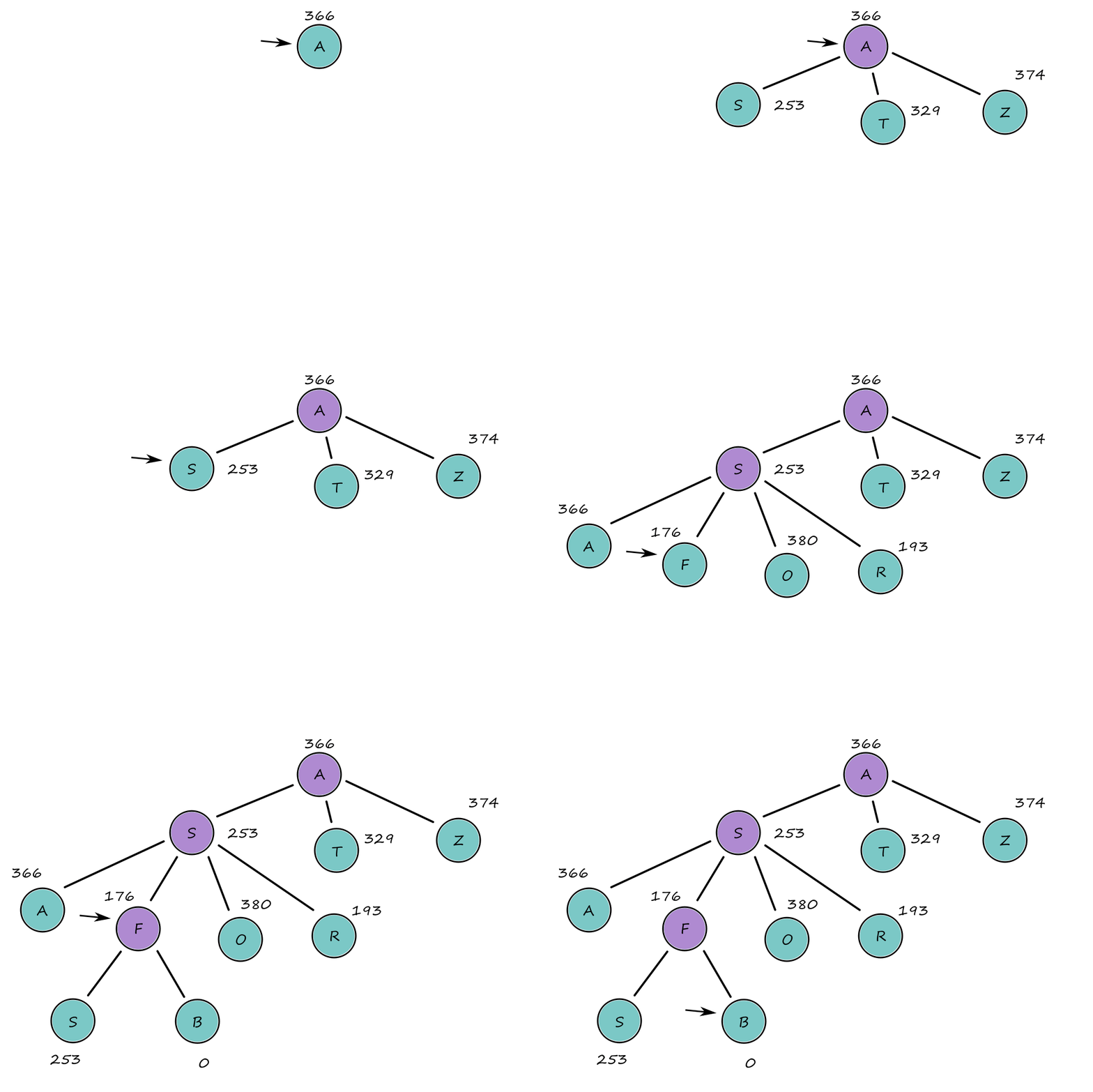
The numbers are the straight-line distances from that node to `B`.
The cost of that path is `450`, but that's not the path with the least cost. The path `A ubrace(rarr)_(140) S ubrace(rarr)_(80) R ubrace(rarr)_(97) P ubrace(rarr)_(101) B` has a lower cost with `418`.
A* Search
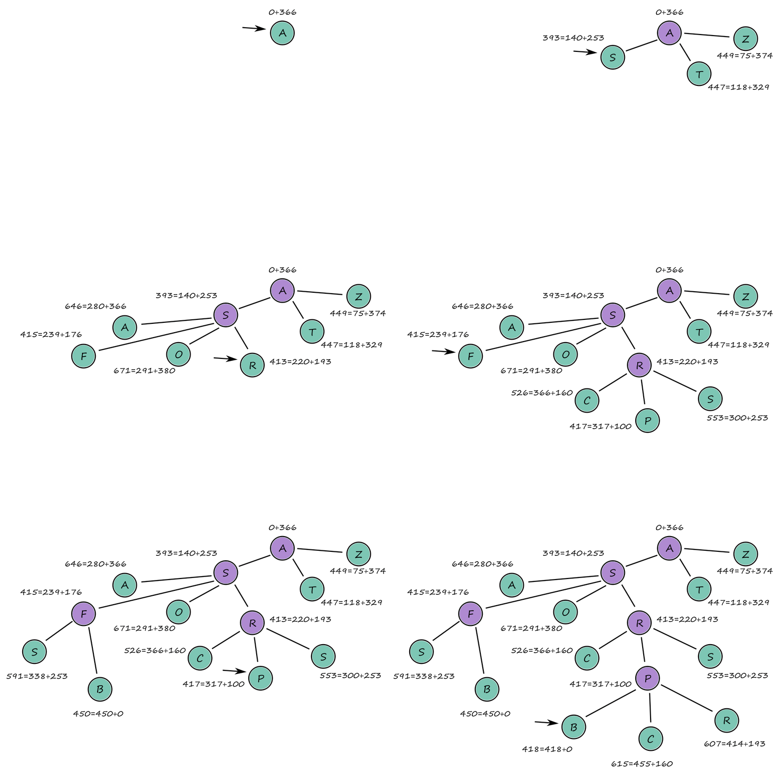
Notice that `B` is found when expanding `F`, but since there's a lower cost available to consider, we don't accept the `F rarr B` path as a solution yet.
A* is efficient because it prunes away nodes that are not necessary for finding an optimal solution. Here, `T` and `Z` are pruned away, but would've been expanded in uniform-cost or breadth-first search.
Recursive best-first search
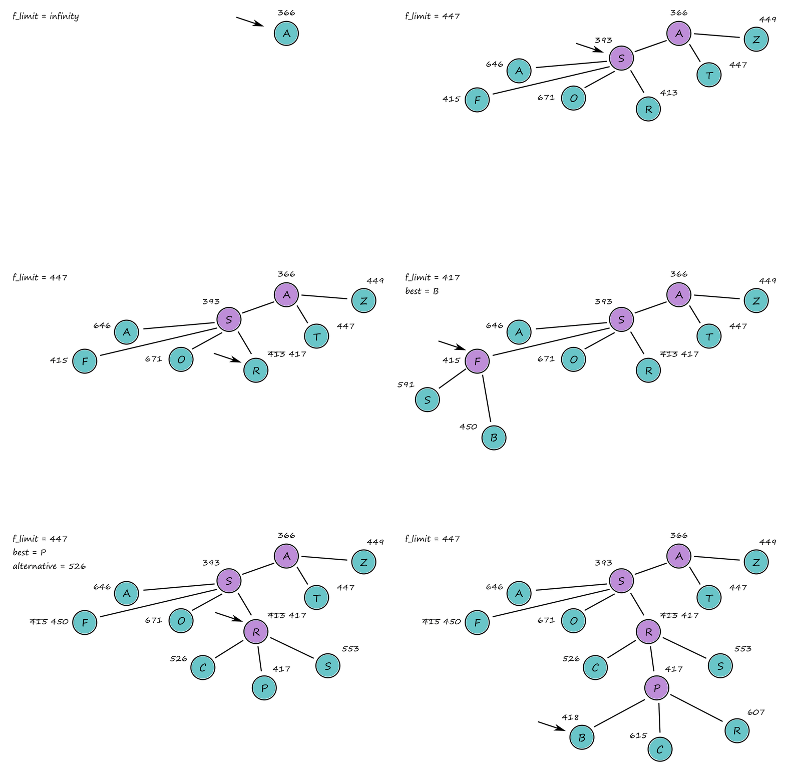
Notice that when `P` is the successor with the lowest `f`-value, `P`'s `f`-value is higher than f_limit. So as we go back up to consider the alternative path, we update `R`'s `f`-value so we can check later if it's worth reexpanding `R`. (The same thing happens for `F`.) The `f`-value that is used as replacement is called the backed-up value, and it's the best `f`-value of the node's children.
RBFS looks similar to A* search in that it looks for the lowest `f`-value. The difference is that RBFS only looks at the `f`-values of the current node's successors while A* search looks at all the nodes in the frontier.
Heuristic Functions
Here, we'll look at how the accuracy of a heuristic affects search performance and how we can come up with heuristics in the first place. We'll use the 8-puzzle as our main example. The 8-puzzle is a `3xx3` sliding-tile puzzle with `8` tiles and `1` blank space. We move tiles horizontally and vertically into the blank space until the goal state is reached (each move has a cost of `1`).
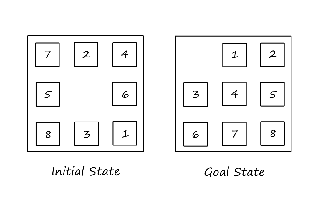
The shortest solution has `26` moves.
Two commonly-used heuristics are
- `h_1=` the number of misplaced tiles (blank space not included)
- for our example, `h_1=8` because all `8` tiles are misplaced
- this is admissible because the number of moves needed to reach a goal state will always be `ge` the number of misplaced tiles
- if all `8` misplaced tiles need just `1` move to get to the correct spot, then the estimated cost is still not overestimated
- `h_2=` the sum of the distances of the tiles from their goal positions
- for our example, `h_2=3+1+2+2+2+3+3+2=18`
- `1` is `3` squares away from its destination, `2` is `1` square away from its destination, `3` is `2` squares away from its destination, ...
- this is sometimes called the city-block distance or Manhattan distance
- this is admissible because the calculation of the distance doesn't take obstacles into account
- `8` is `2` squares away from its destination, but it may actually need `ge 2` moves
- for our example, `h_2=3+1+2+2+2+3+3+2=18`
The effect of heuristic accuracy on performance
One way to assess the quality of a heuristic is to look at the effective branching factor `b^(**)`. It can loosely be thought of as the average number of nodes that are generated at each depth. A good heuristic would have `b^(**)` close to `1`, which means that not a lot of nodes are being generated the farther we go down a path (we're fairly successful in finding good paths).
If A* finds a solution at depth `5` using `52` nodes, then the effective branching factor is `1.92`.
It turns out that `h_2` (the Manhattan distance) is always better than `h_1` (the number of misplaced tiles). This means that `h_2` dominates `h_1`. Because of this, A* search using `h_2` will never expand more nodes than A* using `h_1` (except for when there are ties).
Earlier we saw that every node with `f(n) lt C^(**)` will surely be expanded (assuming consistent heuristic).
`f(n) lt C^(**)`
`g(n)+h(n) lt C^(**)`
`h(n) lt C^(**)-g(n)`
So every node with `h(n) lt C^(**)-g(n)` will surely be expanded. By definition, `h_2(n) ge h_1(n)`, so every node that is surely expanded by A* with `h_2` is also surely expanded by A* with `h_1`. Mathematically, this is because `h_1(n) le h_2(n) lt C^(**)-g(n)`. But because `h_1` is small, there are more nodes that are `lt C^(**)-g(n)`, so A* with `h_1` will expand other nodes that A* with `h_2` wouldn't have expanded.
So it's generally better to use a heuristic function with higher values, assuming it's consistent and it's not too computationally intensive.
Generating heuristics from relaxed problems
So how do we come up with heuristics like `h_1` and `h_2` in the first place? (Perhaps more importantly, is it possible for a computer to come up with such a heuristic?)
Let's make the 8-puzzle simpler so that tiles can be moved anywhere, even if there's another tile occupying the spot. Notice now that `h_1` would give the exact length of the shortest solution.
Let's consider another simplified version where the tiles can still only move `1` square but, now, in any direction, even if the square is occupied. Notice that `h_2` would give the exact length of the shortest solution.
These simplified versions, where there are fewer restrictions on the actions, are relaxed problems. The state-space graph of a relaxed problem is a supergraph of the original state space because the removal of restrictions allows for more possible states, resulting in more edges being added. This means that an optimal solution in the original problem is also an optimal solution in the relaxed problem. But the relaxed problem may have better solutions (this happens when the added edges provide shortcuts).
That last part is how we can come up with heuristics. The cost of an optimal solution to a relaxed problem is an admissible heuristic for the original problem. (Also, if the heuristic is an exact cost for the relaxed problem, it must obey the triangle inequality, making it consistent.)
So how can we come up with relaxed problems systematically?
Let's describe the 8-puzzle actions as follows: a tile can move from square `X` to square `Y` if `X` is adjacent to `Y` and `Y` is blank. From this, we can generate three relaxed problems simply by removing one or both of the conditions:
- A tile can move from square `X` to square `Y` if `X` is adjacent to `Y`
- A tile can move from square `X` to square `Y` if `Y` is blank
- A tile can move from square `X` to square `Y`
From the first one, we can derive `h_2` (the Manhattan distance) and from the third one, we can derive `h_1` (the number of misplaced tiles).
Ideally, relaxed problems generated by this technique should be solveable without search.
If we generate a bunch of relaxed problems, we now also have a bunch of heuristics. If none of them are much better than the others, then which one should be used? One thing we can do is to pick the heuristic that gives the highest value:
`h(n)=max{h_1(n), ..., h_k(n)}`
But if it takes too long to compute all the heuristics, then we can also randomly pick one or use machine learning to predict which heuristic will be the best.
Generating heuristics from subproblems: Pattern databases
Let's consider a subproblem of the 8-puzzle, where the goal is to get only tiles `1,2,3,4,` and the blank space into the correct spots.
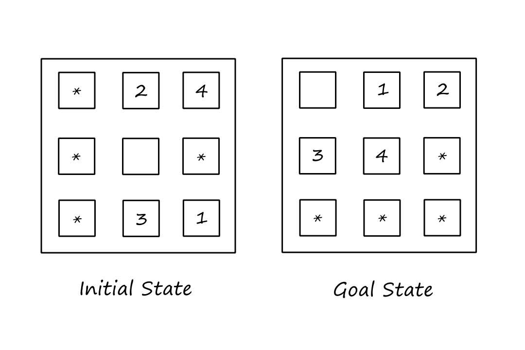
Since there are fewer tiles that have to be in a certain spot, the cost of the optimal solution of this subproblem is a lower bound on the cost of the complete problem, meaning that this could make a good admissible heuristic.
For every possible subproblem, we can store the exact costs of their solutions in a pattern database. So when we're trying to solve the complete problem, we could look in our database for the subproblem that matches our current state and use the exact cost of the subproblem as the heuristic for the complete problem.
We could have multiple databases for each subproblem type. For example, one database could be all the subproblem instances with tiles `1,2,3,4`. Another database could be all the subproblem instances with tiles `5,6,7,8`. Another database could be all the subproblem instances with tiles `2,4,6,8`. And so on. Then the heuristics from these databases can be combined by taking the maximum value. Doing this turns out to be more accurate than the Manhattan distance.
Generating heuristics with landmarks
This is kinda similar to using pattern databases, but kinda makes more sense when viewed in the context of route-finding problems.
We can pick a few landmark points and precompute the optimal costs to these landmarks. More formally, for each landmark `L` and for each other vertex `v` in the graph, we compute and store `C^(**)(v,L)`. This may sound time-consuming, but it only needs to be done once and it will be infinitely useful.
So if we're trying to estimate the cost to the goal, we can look at the cost to get there from a landmark.
The heuristic would be
`h_L(n)=min_(L in text(landmarks)) C^(**)(n,L)+C^(**)(L,text(goal))`
This heuristic is inadmissible though. If the optimal path is through a landmark, then this heuristic will be exact. If it isn't, then it will overestimate the optimal cost (the exact cost of a non-optimal path is greater than the exact cost of an optimal path).
However, we can come up with an admissible heuristic:
`h_(DH)(n)=max_(L in text(landmarks)) abs(C^(**)(n,L)-C^(**)(L,text(goal)))`
This is a differential heuristic (differential because of the subtraction). To understand it intuitively, consider a landmark that is beyond the goal. If the goal happens to be on the optimal path to the landmark, then the path `n rarr text(goal) rarr L` minus the path `text(goal) rarr L` gives us the optimal path `n rarr text(goal)`.
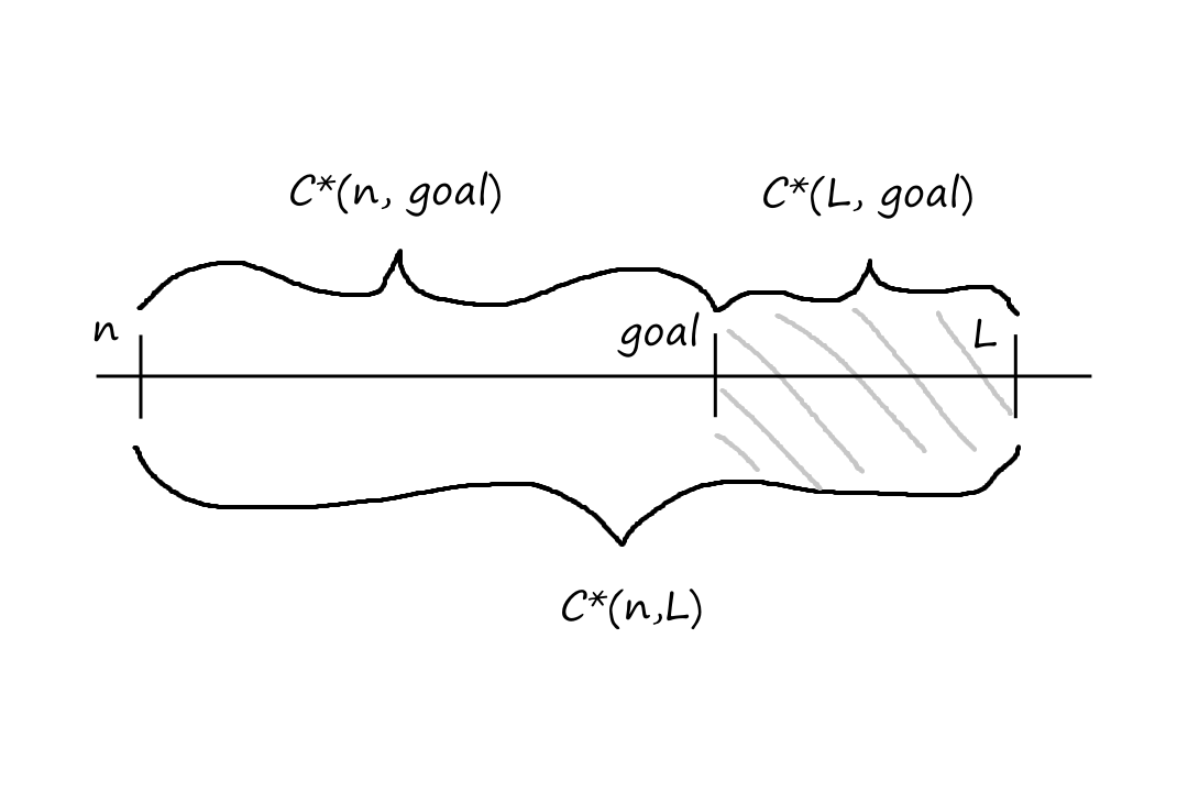
If the goal is not on the optimal path to the landmark, then we would be subtracting by a larger value, resulting in a cost `lt` the optimal cost, i.e., the cost is underestimated.
Landmarks that are not beyond the goal will already underestimate the cost to the goal, but these landmarks are not likely to be considered since we're selecting the max.
A good way to decide landmark points are by looking at user requests for frequently requested landmarks.
Learning heuristics from experience
Sometimes, we can just develop an intuition for something if we do it many times. From the perspective of computers, they can pick up on patterns in past data and come up with a heuristic that seems to align with those patterns. A lot of this seems to depend on luck, so the heuristics are not expected to be admissible (much less consistent).
For example, the number of misplaced tiles might be helpful in predicting the actual cost. For further example, we might find that when there are `5` misplaced tiles, the average solution cost is around `14`.
Another feature that might be useful is the number of pairs of adjacent tiles that are not adjacent in the goal state.
If we have multiple features, we can combine them to generate a heuristic by using a linear combination of them:
`h(n)=c_1x_1(n)+c_2x_2(n)+...+c_kx_k(n)`
where each `x_i` is a feature
Machine learning would be used to figure out the best values for the constants.
Summary of Chapter 3
- A well-defined search problem consists of five parts: the initial state, a set of actions, a transition model that describes the results of those actions, a set of goal states, and an action cost function.
- The environment of the problem is represented by a state space graph. A path through the state space from the initial state to a goal state is a solution.
- Uninformed search methods have access only to the problem definition. Algorithms build a search tree to find a solution but differ based on which node they expand first.
- Best-first search expands the node with the lowest value given by an evaluation function.
- Breadth-first search expands the shallowest nodes first. It is complete, optimal for unit action costs, but has exponential space complexity.
- Uniform-cost search expands the node with the lowest path cost, `g(n)`, and is optimal for general action costs.
- Depth-first search expands the deepest unexpanded node first. It is neither complete nor optimal, but has linear space complexity. Depth-limited search adds a depth bound.
- Iterative deepening search calls depth-first search with increasing depth limits until a goal is found. It is complete when full cycle checking is done, optimal for unit action costs, has exponential time complexity, and has linear space complexity.
- Bidirectional search expands two frontiers, one around the initial state and one around the goal, stopping when the two frontiers meet.
- Informed search methods have access to a heuristic function `h(n)` that estimates the cost of a solution from `n`.
- Greedy best-first search expands the node with the lowest value of `h(n)`. It is not optimal but is often efficient.
- A* search expands the node with the lowest value of `f(n)=g(n)+h(n)`. It is complete and optimal (if `h(n)` is admissible), but uses up a lot of space.
- IDA* (iterative deepening A* search) is an iterative deepening version of A* that addresses the space complexity issue.
- RBFS (recursive best-first search) is a robust, optimal search algorithm that uses limited amounts of memory.
- Beam search puts a limit on the size of the frontier. This makes it incomplete and suboptimal, but it often finds reasonably good solutions and is generally faster than complete searches.
- Weighted A* search expands fewer nodes but sacrifices optimality.
- The performance of heuristic search algorithms depends on the quality of the heuristic function.
- Good heuristics can be obtained by relaxing the problem definition, by storing precomputed solution costs for subproblems in a pattern database, by defining landmarks, or by learning from experience.
Earlier, we assumed that the environments are episodic, single agent, fully observable, deterministic, static, discrete, and known. Now we'll start relaxing these constraints to get closer to the real world.
Local Search and Optimization Problems
There are some search problems where we only care about what a goal state looks like (and we don't care what the path looks like). For example, the 8-queens problem is to find a valid placement of 8 queens such that no queens are attacking each other. Once we know what a solution looks like, it's trivial to reconstruct the steps to get there.
Local search algorithms work without keeping track of the paths or the states that have been reached. This means that they don't explore the whole search space systematically, i.e., they are not complete and may not find a solution. However, they use very little memory and can find reasonable solutions in problems with large or infinite state spaces.
Local search also works for optimization problems, where the goal is to find the best state according to some objective function. The objective function represents what we're trying to maximize/minimize.
Hill-climbing search
Let's take a look at a sample state-space landscape.
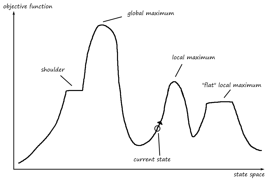
One goal might be to find the highest peak, which is the global maximum. This process is called hill climbing.
If the goal is to find the lowest valley (global minimum), then the process is called gradient descent.
The hill climbing search algorithm is pretty simple. It keeps moving forward until the next state it finds has a smaller value than the value of the current state.
function HILL-CLIMBING(problem)
  current = problem.INITIAL
  while true do
    neighbor = a highest-valued successor state of current
    if VALUE(neighbor) ≤ VALUE(current) then return current
    current = neighbor
This particular version of hill climbing is steepest-ascent hill climbing because it heads in the direction of the steepest ascent.
Hill climbing is sometimes also called greedy local search because it gets a good neighbor state without thinking ahead about where to go next.
There are some situations where the hill climbing algorithm can get stuck before finding a solution. One situation is when a local maximum is reached. In this situation, every possible move results in a worser state.
Another situation is when a plateau is reached. A plateau can be a flat local maximum or a shoulder, where there is an uphill exit. In this situation, every possible move doesn't result in a better state (except if the plateau is a shoulder and we're right at the edge of the uphill exit).
Let's look at the problem of positioning hospitals so that they are as close as possible to every house.

The cost is the sum of the distances from each house to the nearest hospital.
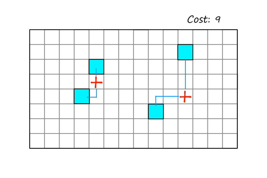
We can see that this is the best way to place the hospitals, but in order to achieve this position, the algorithm has to make the move below first.
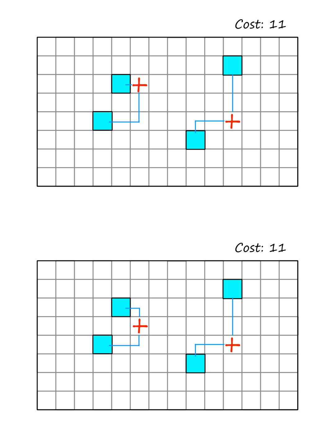
Since this move doesn't result in a better state, the hill climbing algorithm won't consider that move. And as a result, the best configuration will never be reached. This is an example of a plateau.
One way to get unstuck is to allow sideways moves, i.e., to allow the algorithm to keep moving as long as the next state isn't worse. The idea is to hope that the plateau is a shoulder. This won't work if the plateau is a local maximum though, in which case we really are stuck.
Another way (kinda) is to just start over, but from a different starting point. This is random-restart hill climbing.
Interestingly, random-restart hill climbing is complete with probability `1` because it will eventually generate a goal state as the initial state.
Stochastic hill climbing chooses a random uphill move instead of the steepest uphill move.
First-choice hill climbing generates successors randomly until one of them is better than the current state.
Simulated annealing
Annealing is the process of hardening metals and glass by heating them to a high temperature and then gradually cooling them.
Sometimes, it's necessary to make worse moves that put us in a temporarily worse state so that we can get to a better position.
function SIMULATED-ANNEALING(problem, schedule) `e^(-DeltaE//T)`
current = problem.INITIAL
for t = 1 to infinity do
T = schedule(t)
if T = 0 then return current
next = a randomly selected successor of current
ΔE = VALUE(current) - VALUE(next)
if ΔE > 0 then current = next
else current = next only with probability
T represents the "temperature", corresponding to the temperature described in annealing.
In the simulated-annealing algorithm, we pick moves randomly instead of picking the best move. If the move puts us in a better situation, then we'll accept it. But if the move puts us in a worse position, then we'll consider it, depending on how bad of a move it is (measured by `DeltaE`). And as time goes on, we'll be less accepting of bad moves.
It's called simulated annealing because the algorithm starts with a high "temperature", meaning that there's a high level of randomness in exploring the search space. As time goes on, the "temperature" gets lower, reducing the random moves.
Local beam search
Local beam search starts with `k` randomly generated states, generates all their successors (if one of them is a goal, then we're done), selects the best `k` successors, and repeats.
Local beam search kinda looks like running `k` random-restart searches in parallel. However, it actually isn't. All random-restart searches are independent of each other, while each local beam search thread passes information to each other.
Evolutionary algorithms
Evolutionary algorithms are based on the ideas of natural selection in biology. There is a population of individuals (states), and the fittest (highest valued) individuals produce offspring (successor states). And just like in real life, the successor states contain properties of the parent states that produced them.
The process of combining the parent states to produce successor states is called recombination. One common way of implementing this is to split each parent at a crossover point and use the four resulting pieces to form two children.
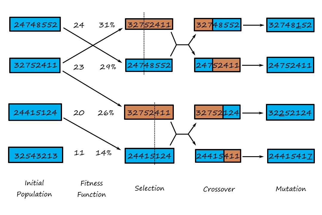
The numbers in the fitness function are sample fitness scores assigned by the fitness function to each state. The fitness scores are then converted to a probability.
Below is an example of how an evolutionary algorithm can be used for the 8-queens problem. We can encode each queen's positions as a number from `1-8`.
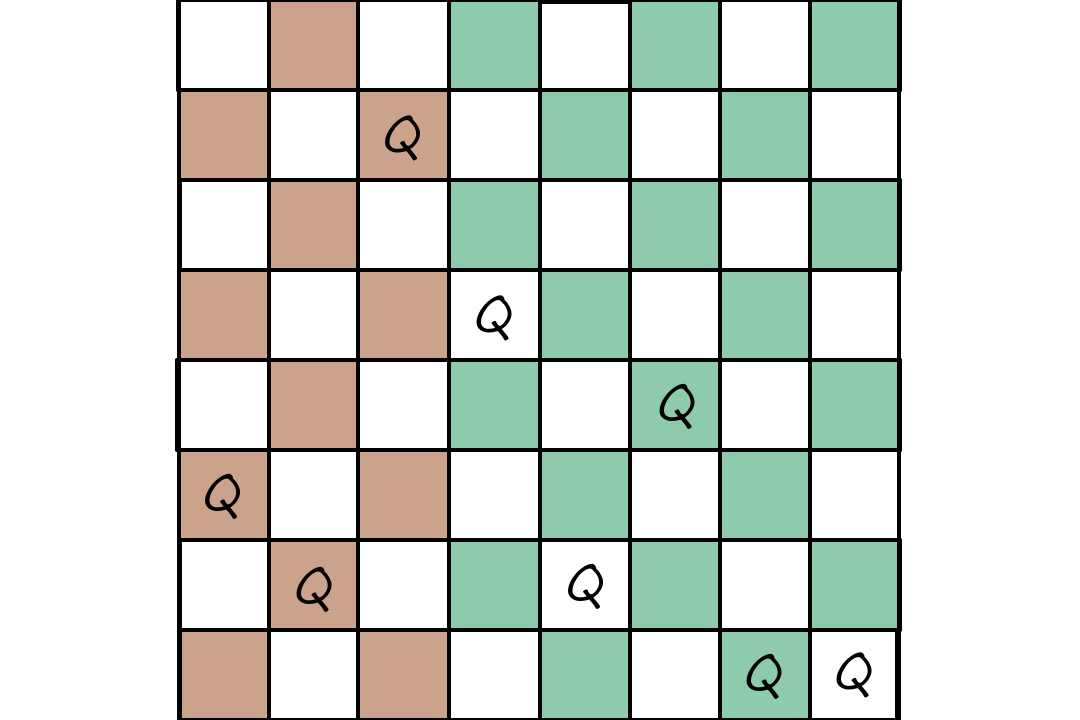
`327|52411`
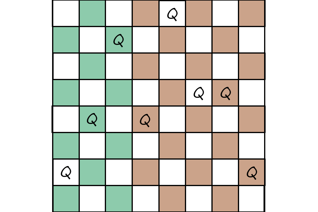
`247|48552`
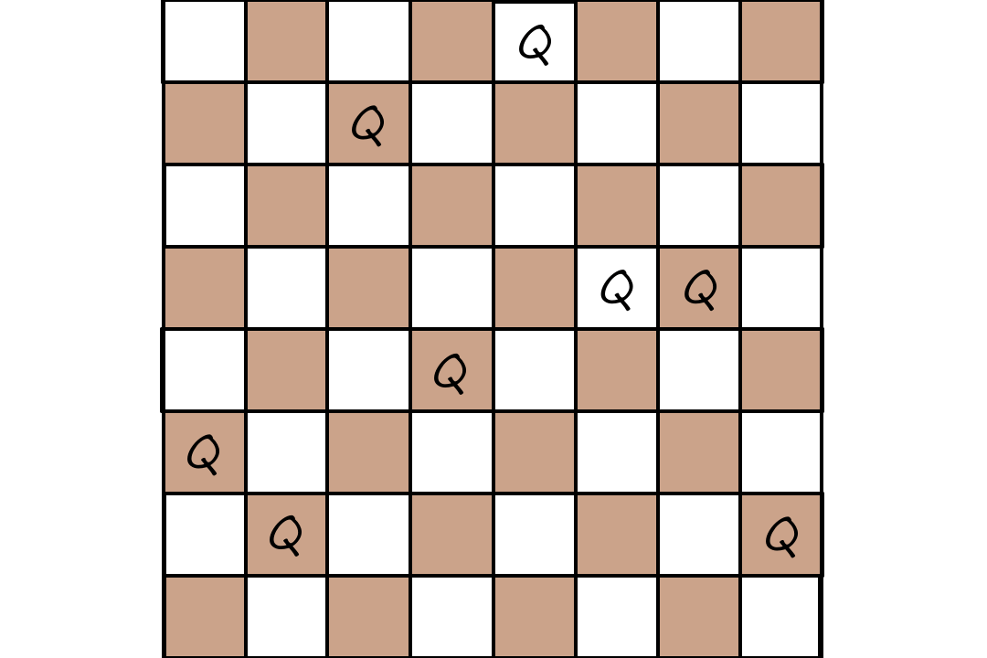
`327|48552`
If we use nonattacking queens as the fitness function, then the sample fitness scores are the number of nonattacking pairs of queens.
Local Search in Continuous Spaces
Most real-world problems take place in a continuous environment, not in a discrete one like the examples we've seen so far. A continuous environment can have a continuous action space (e.g., a robotic arm moving anywhere between `0` and `180` degrees), a continuous state space (e.g., the current position of a robot in a room), or both.
A continuous action space has an infinite branching factor, so most of the algorithms we've seen so far won't work (except for first-choice hill climbing and simulated annealing).
One way to deal with a continuous state space is to discretize it.
For example, suppose we want to place three new airports in an area such that each city is as close as possible to its nearest airport. The state space is defined by the coordinates of the three airports: `(x_1, y_1),(x_2, y_2),(x_3, y_3)`. To discretize this, we could predefine fixed points on a grid and only allow the airports to be at those fixed points.
One way to deal with a continuous action space is to choose successor states randomly by moving in a random direction by a small amount. As we move, we look at how the value of the objective function changes to see if we're going in the right direction. This is empirical gradient search.
Steepest-ascent hill climbing can be seen as a specific case of empirical gradient search when the state space is discretized.
The objective function for any particular state is
`f(x_1, y_1, x_2, y_2, x_3, y_3) = sum_(i=1)^3sum_(c in C_i)(x_i-x_c)^2+(y_i-y_c)^2`
Note that this objective function is only correct locally, not globally. As the location of an airport moves, the closest cities to that airport change and have to be recomputed.
As in the example above, the objective function can often be expressed in a math equation. This means that we can use calculus to find the steepest ascent rather than moving randomly to try and find it.
For the above objective function, the gradient is calculated by
`grad f = ((del f)/(del x_1),(del f)/(del y_1),(del f)/(del x_2),(del f)/(del y_2),(del f)/(del x_3),(del f)/(del y_3))`
Search with Nondeterministic Actions
Now, we'll look at nondeterministic environments. When the environment is nondeterministic, the agent doesn't know for sure what state it will end up in after performing an action. So the agent will be thinking something like, "If I do action `a` I'll end up in state `s_2`, `s_4`, or `s_5`. The states that the agent believes are possible are called belief states.
Instead of a sequence of states, the solution to a problem is a conditional plan that specifies what to do depending on the situation.
The erratic vacuum world
We're going back to our vacuum world! But this time, our vacuum is a little unpredictable. When it cleans a dirty square, it can sometimes clean an adjacent square as well. If it cleans a clean square, it can sometimes deposit dirt on it.
AND-OR search trees
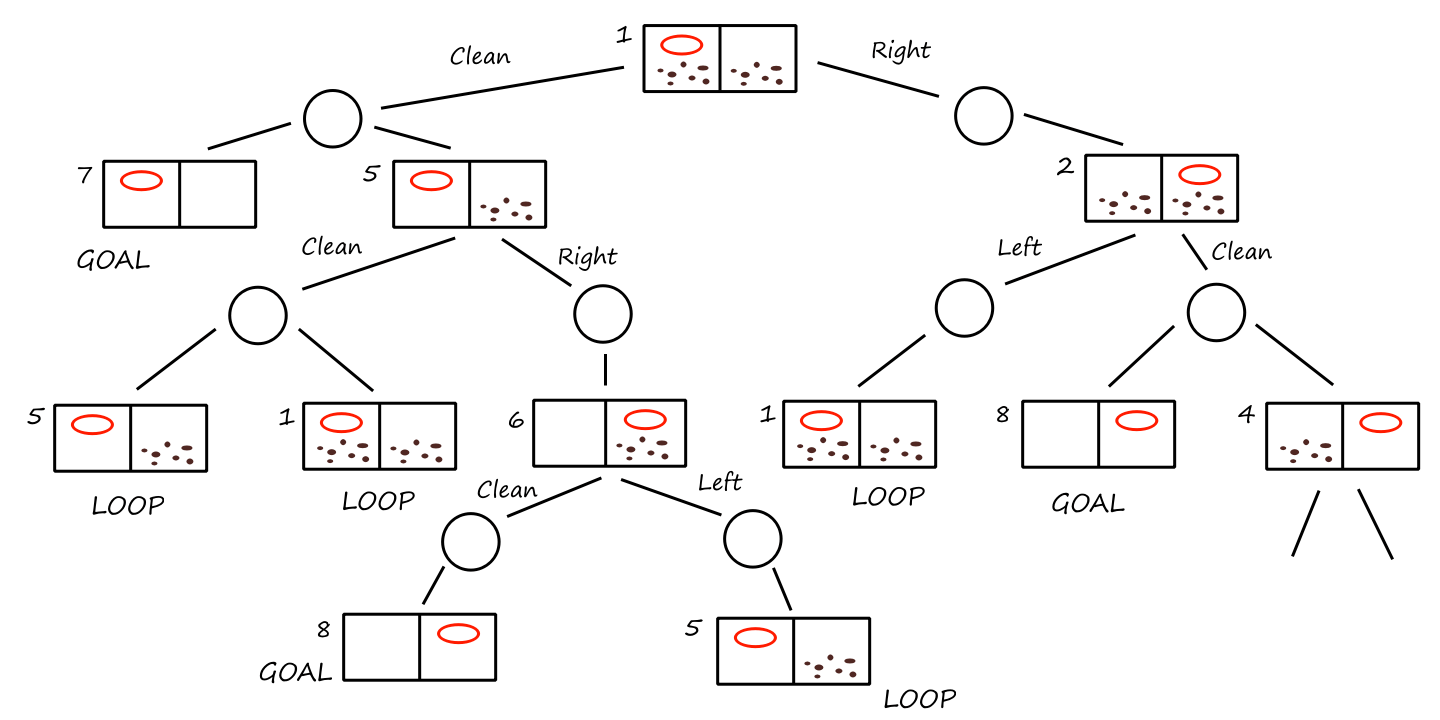
Yes, the red oval is our vacuum cleaner. The states are labeled from `1-8`.
Notice that there's no single sequence of actions that can solve the problem. But this conditional plan does:
[Clean, if State == 5 then [Right, Clean] else []]
As the name suggests, an AND-OR search tree has OR nodes and AND nodes. OR nodes (represented as rectangles in the example above) are thought of as, "at this node, I can do this or that". AND nodes (represented as circles) are thought of as, "at this node, this and this can happen".
function AND-OR-SEARCH(problem)
  return OR-SEARCH(problem, problem.INITIAL, [])
function OR-SEARCH(problem, state, path)
  if problem.IS-GOAL(state) then return empty plan
  if IS-CYCLE(path) return faliure
  for each action in problem.ACTIONS(state) do
    plan = AND-SEARCH(problem, RESULTS(state, action), [state] + path)
    if plan != failure then return [action] + plan
  return failure
function AND-SEARCH(problem, states, path)
  for each s_i in states do
    plan_i = OR-SEARCH(problem, s_i, path)
    if plan_i == failure then return failure
  return [if s_1 then plan_1 else if s_2 then plan_2 else ...if s_n-1 then plan_n-1 else plan_n]
This is a recursive, depth-first algorithm for AND-OR graph search.
One thing to note is that we're returning failure when there's a cycle. This doesn't mean that a cycle implies no solution. It means that if there is a solution, it should exist on a path before the cycle, so there's no point in continuing to explore this path. This also ensures that the algorithm doesn't run infinitely.
Try, try again
Forget our erratic vacuum for a moment. Let's go back to our normal vacuum, but this time, the floor is slippery. So sometimes, when the vacuum tries to move, it stays in place instead.
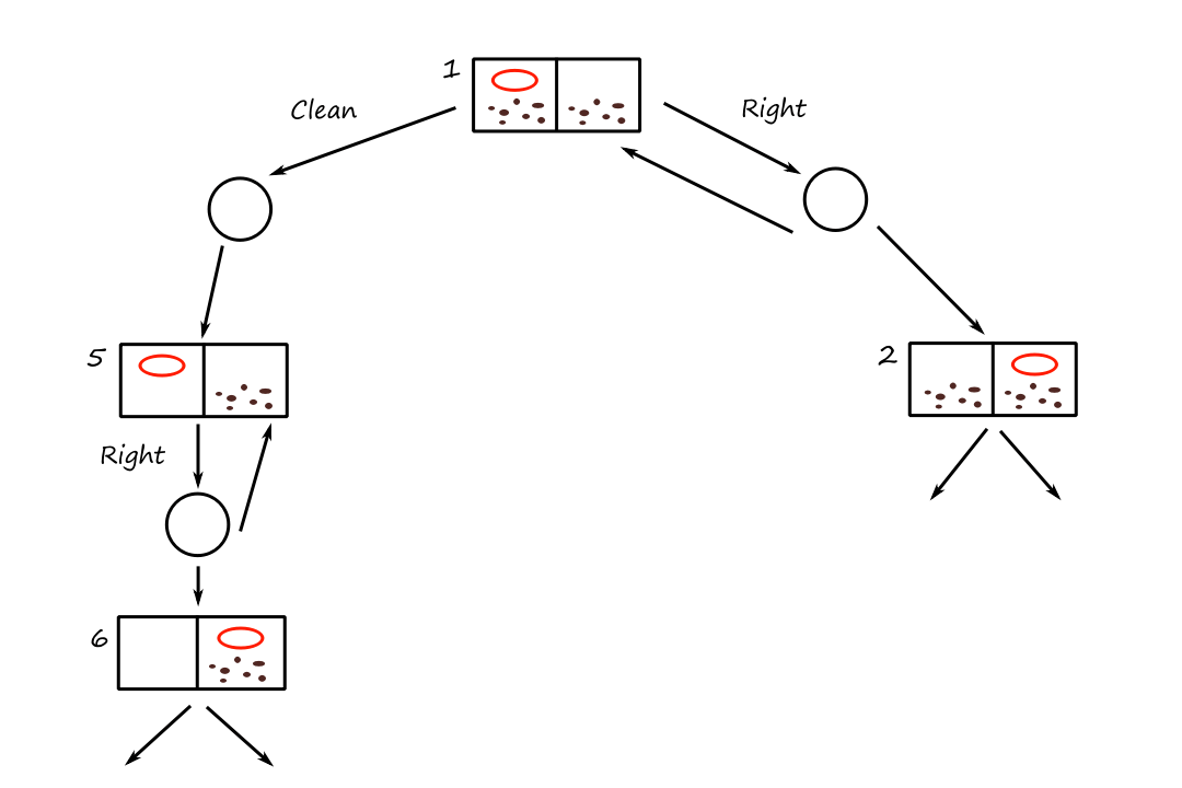
Here, if we're in state `5` and the vacuum moves right, it can either move right or stay in place. If it stays in place, we still want it to move right. So the solution here is to keep moving right until it works.
[Clean, while State == 5 do Right, Clean]
This is a cyclic plan that happens to also be a solution, i.e., a cyclic solution.
Search in Partially Observable Environments
Now, we'll look at what happens when the environment is partially observable. When the environment is partially observable, the agent doesn't know for sure what state it's in. So the agent will be thinking something like, "I'm either in state `s_1` or `s_3`".
Searching with no observation
If the agent has no sensors at all, then the problem that the agent is trying to solve is called a sensorless problem. It might seem impossible for an agent to be able to do anything without sensors, but, in fact, there are sensorless solutions that are common and useful because they don't rely on sensors working properly.
So let's go back to when the vacuum was working normally. Except, the vacuum now has no sensors, so it doesn't know its own location or which squares have dirt (including the square it's currently on). But let's say the vacuum knows what all the possible states look like.
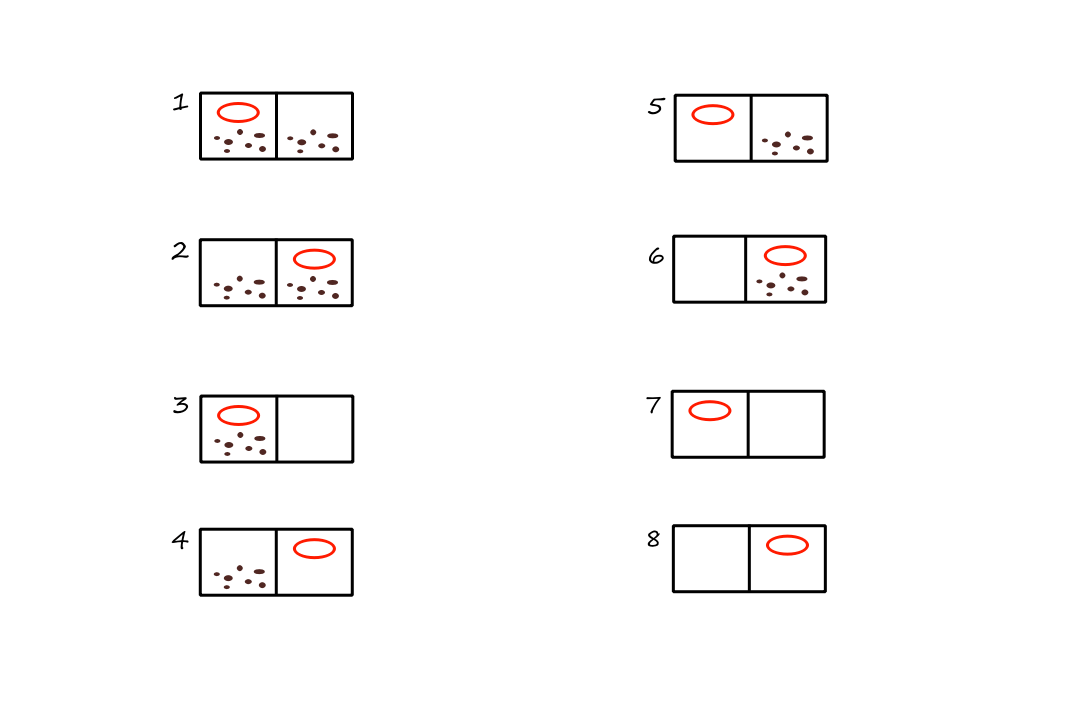
When it starts out, the vacuum's initial belief state is `{1, 2, 3, 4, 5, 6, 7, 8}`. No matter what state it's in, if the vacuum moves right, then it will be in one of the states `{2, 4, 6, 8}`. After cleaning, it will be in `{4,8}`. Then after moving left and cleaning, it will be in state `7`. So no matter what state the vacuum starts in, we can coerce the world into state `7` with [Right, Clean, Left, Clean].
The solution to a sensorless problem is a sequence of actions, not a conditional plan. This is because the agent can't sense anything, and thus, can't tell when it needs to go with another plan.
So the solutions can be found by using the informed and uninformed search algorithms from before. We just have to search in the space of belief states instead of physical states.
In belief-state space, the problem is fully observable because combining all the information about what states the agent could be in provides the agent with a complete picture of the environment.
If we transform a physical problem `P` (with `text(Actions)_P`, `text(Result)_P`) into a belief-state problem, we have:
- states: every possible subset of physical states
- if `P` has `N` states, then the belief-state problem has `2^N` belief states
- note that this is not saying that a belief state has `2^N` physical states
- if `P` has `N` states, then the belief-state problem has `2^N` belief states
- initial state: usually, the belief state consisting of all states in `P`
- goal test: all states in the current belief state must be a goal state
- action cost: to simplify things, we'll assume the cost of an action is the same in all states
Defining the actions is a little more involved. A belief state can have multiple physical states, so there can be multiple actions available from each state. Inherently, there can be some actions that are possible in some of the states but not others. If illegal actions don't have an effect on the environment, then we can combine all the actions from each state and say that those are the available actions for the current belief state. Otherwise, we can find the actions that are common in all the states and say that those are the available actions.
For example, in our vacuum world, let's say the belief state is `{s_1, s_2}`. All the possible actions from both states are to move left, move right, and clean. However, it's not really useful for a vacuum in `s_1` to move left. We've been assuming that if the vacuum can't move in a certain direction, it just stays still. So in this case, it's okay to combine all the actions and say that the available actions for `{s_1,s_2}` are to move left, move right, and clean.
On the other hand, if the vacuum can fall off the edge, then we don't want it to move left if it's in `s_1`. Likewise, we don't want it to move right if it's in `s_2`. The only action in common from all states is to clean, so the available actions for the belief state in this case would be to just clean.
`text(Actions)(b)=uuu_(s in b) text(Actions)_P(s)` or `text(Actions)(b)=nnn_(s in b) text(Actions)_P(s)` depending on which makes sense.
Defining the transition model is also a little more involved depending on whether the actions are deterministic or not. For deterministic actions, there is one result state for each of the states in the belief state. For nondeterministic actions, it's the combination of all the possible result states for each of the states.
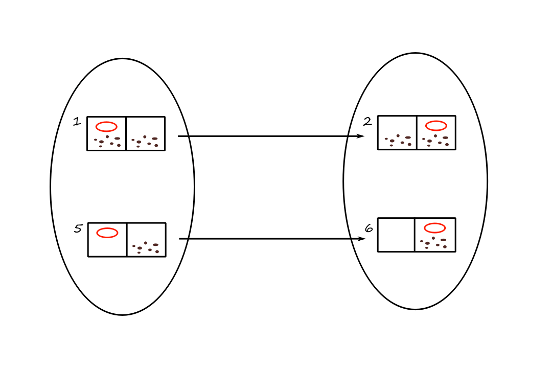
The transition model for moving right in the normal vacuum world.
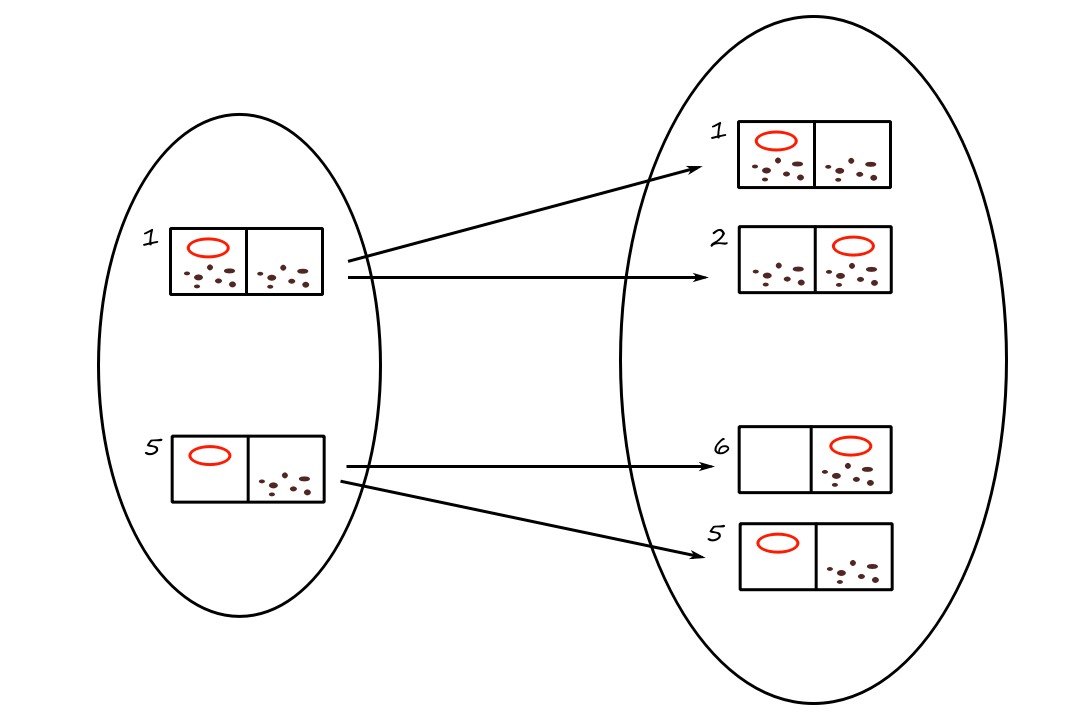
The transition model for moving right in the slippery vacuum world.
deterministic: `b' = text(Result)(b,a)={s' : s' = text(Result)_P(s,a) and s in b}`
nondeterministic: `b' = text(Result)(b,a)={s' : s' in text(Results)_P(s,a) and s in b} = uuu_(s in b)text(Results)_P(s,a)`
By transforming a physical problem into a belief-state problem with these definitions, we can use the informed and uninformed search algorithms to find a solution. The operative word being "can". As mentioned earlier, there are a total of `2^N` possible belief states to search through. Furthermore, a belief state can have up to `N` states, so it can be hard to store multiple belief states in memory.
An alternative is to use incremental belief-state search algorithms. For example, if the initial belief state is `{1,2,3,4,5,6,7,8}`, we can start by finding a solution for state `1` and see if it works for every other state. If it doesn't, then we go back to state `1`, find another solution, and repeat until the solution works for all `8` states.
Searching in partially observable environments
Now we'll upgrade our vacuum to have local sensors that can tell it which square it's on and whether it's clean or dirty. Suppose the vacuum gets the information [L, Dirty] from its sensors. From this, the vacuum can either be in state `1` or state `3`. So it's belief state will be `{1,3}`.
The transition model between belief states can be seen as a three-stage process:
- prediction stage: see what states are possible from performing on action on the current belief state
- possible percepts stage: see what percepts are possible from each of the states
- update stage: compute the belief states that are possible based on the possible percepts
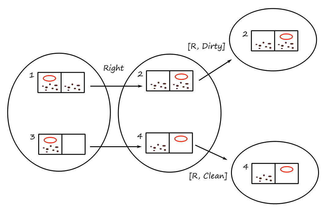
The transition model for moving right in the normal (local sensing) vacuum world.
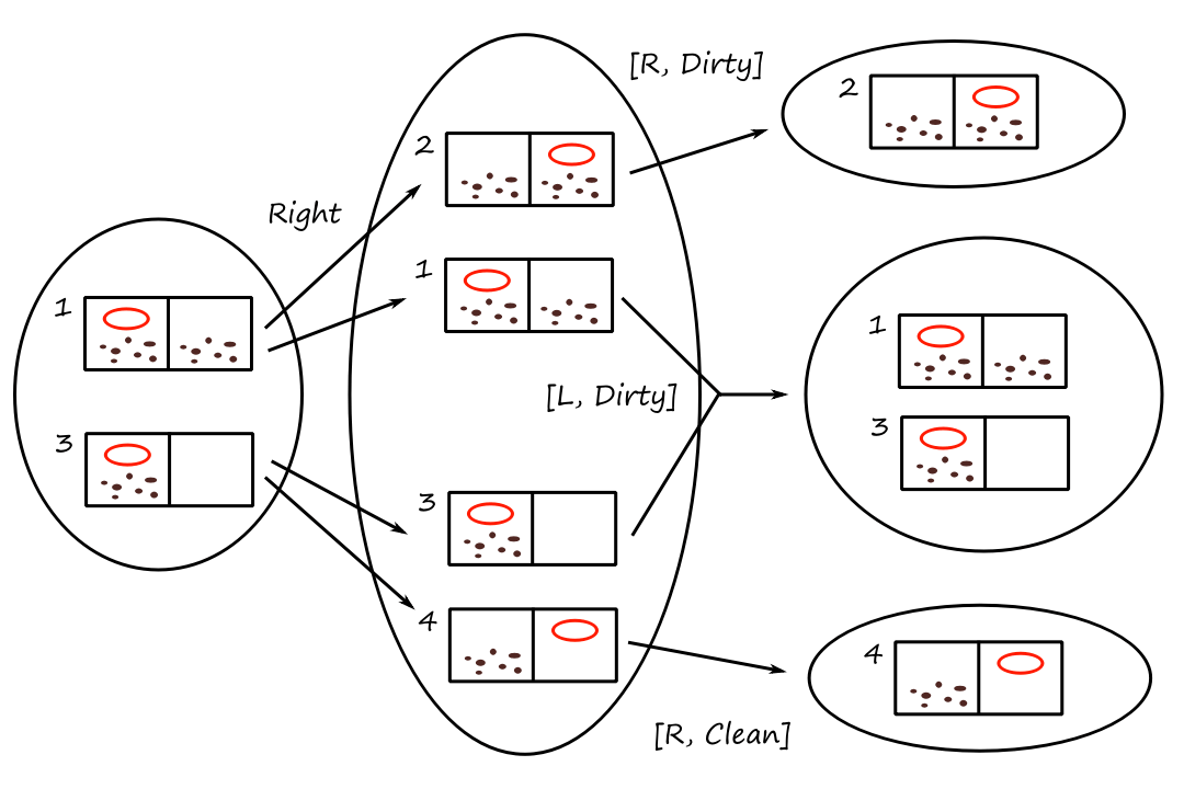
The transition model for moving right in the slippery (local sensing) vacuum world.
prediction stage: `hat b = text(Result)(b,a)` (the `text(Result)` function can also be called `text(Predict)`)
possible percepts stage: `text(Possible-Percepts)(hat b) = {o : o = text(Percept)(s) and s in hat b}`
update stage: `text(Update)(hat b,o) = {s : o = text(Percept)(s) and s in hat b}`
transition model: `text(Results)(b,a) = {b_o : b_o = text(Update)(text(Predict)(b,a), o) and o in text(Possible-Percepts)(text(Predict)(b,a))}`
Solving partially observable problems
Because the current belief state can yield multiple belief states as the next possible states, we can treat the multiple belief states as if they were the result of a nondeterministic action and, therefore, use the AND-OR search algorithm. As a result, the solution is a conditional plan. For example, [Clean, Right, if state == 6 then Clean else []] is a solution to the search tree below.
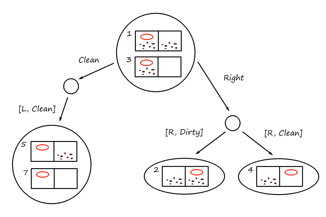
Remember that the transition model returns one belief state per possible percept.
Online Search Agents and Unknown Environments
In this context, online isn't referring to the Internet. An online search agent makes an action, observes the environment, and computes the next action. As opposed to an offline search agent that computes a complete solution first before taking any action. Mostly everything we've seen so far has been offline search algorithms.
Online search is good for (semi-)dynamic environments where the agent can't sit around doing nothing for too long. It's also good for nondeterministic environments because it allows the agent to focus on the percepts that it actually receives rather than the percepts that it can receive.
On the flip side, more planning reduces the chances of things going wrong.
We'll briefly return to deterministic and fully observable environments here.
Online search problems
The agent only knows the actions that are available in the current state, the cost of going to the next state (once the next available states have been computed), and whether or not the current state is a goal state. The agent cannot know the result of going to another state until it's in that state. The agent might have access to a heuristic function.
An online algorithm can only generate successors for the state that it's currently in. On the other hand, offline algorithms, such as A* search, can expand a node in one part of the space and then immediately expand a node in a distant part of the space.
Online explorers are vulnerable to dead ends, which are states from which no goal state is reachable. Dead ends are a result of irreversible actions, i.e., actions that prevent returning to the previous state.
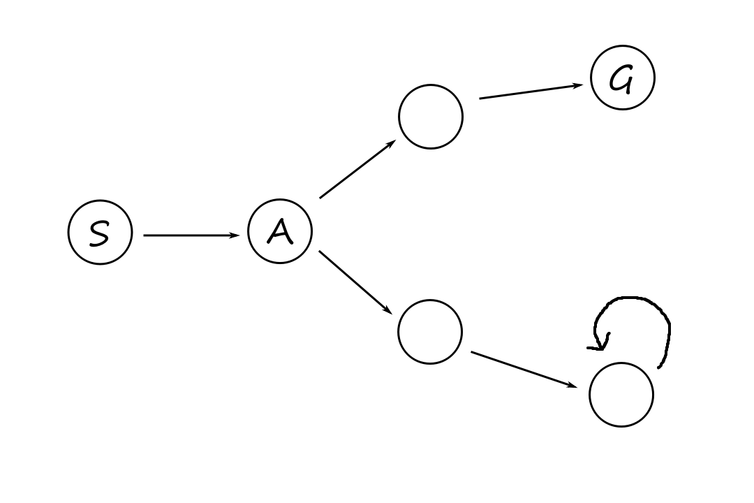
An environment with no dead ends is safely explorable, which means that a goal state is reachable from every reachable state. Any environment with only reversible actions are safely explorable.
function ONLINE-DFS-AGENT(problem, s')
  if problem.IS-GOAL(s') then return stop
  if s' is a new state (not in untried) then untried[s'] = problem.ACTIONS(s')
  if s is not null then
    result[s,a] = s'
    add s to the front of unbacktracked[s']
  if untried[s'] is empty then
    if unbacktracked[s'] is empty then return stop
    else a = an action b such that result[s',b] = POP(unbacktracked[s'])
  else a = POP(untried[s'])
  s = s'
  return a
result: a table mapping `(s,a)` to `s'`
untried: a table mapping `s` to a list of untried actions
unbacktracked: a table mapping `s` to a list of states never backtracked to
Online local search
Since hill-climbing search just keeps the current state in memory, it's actually already an online search algorithm. It's not a very good one though because it can result in agents getting stuck at a local maximum. And random-restart hill climbing is not an option to get unstuck because the agent can't teleport to a new start state.
A random walk can be used to explore an environment. The agent selects an action at random and performs it.
Random walks are complete when the space is finite and safely explorable.
Instead of telling the agent to do random things, we can have the agent learn about its environment as it explores it. One way to do this is to store a "current best estimate" of the cost to reach the goal from each state that has been visited.
The current best estimate, denoted as `H(s)`, starts out being just the heuristic `h(s)`, but it gets updated as the agent learns more.
Consider this sample state space. `(a),(b),(c),(d),(e)` are five iterations of an algorithm called learning real-time A* (LRTA*) search that implements this current best estimate idea. If we look at `(a)`, we see that the agent is currently stuck in a local minimum.
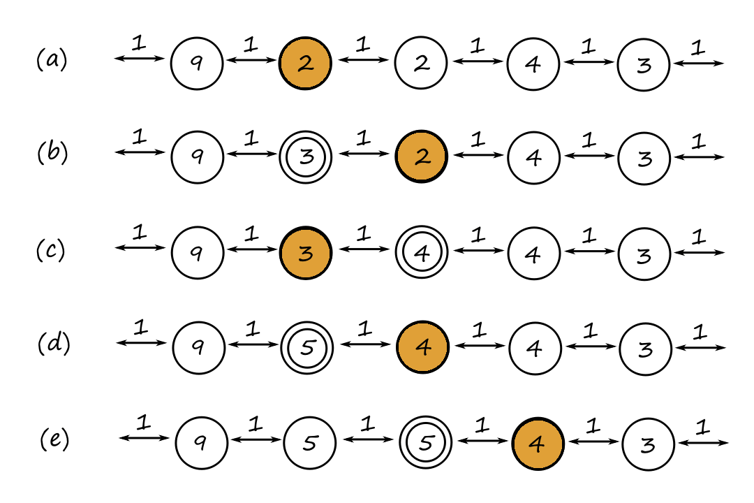
Each state is labeled the current estimated cost to reach a goal (`H(s)`). Every action costs `1`.
The orange state is the agent's current location. The double-circled states are states that have had their cost estimates updated.
At `(a)`, there are two actions: move left or move right. The estimated cost to reach a goal if we move left is `1+9=10` and the estimated cost to reach a goal if we move right is `1+2=3`. So we move right. Importantly, we also update the previous state's estimated cost with the lowest one (`3` vs `10`).
At `(b)`, the estimated cost to the goal if we move left is `1+3=4` and the estimated cost to the goal if we move right is `1+4=5`. We move left and update the previous state's estimated cost (`4` vs `5`).
We can eventually see that we get unstuck (and "flatten out" the local minimum in the process).
LRTA* is complete when the environment is finite and safely explorable. However, unlike A*, it is not complete if the state space is infinite.
Summary of Chapter 4
- Local search methods such as hill climbing keep only a small number of states in memory. They have been applied to optimization problems, where the idea is to find a high-scoring state without worrying about the path to that state.
- Simulated annealing is a stochastic local search algorithm that returns optimal solutions when given an appropriate cooling schedule.
- Local search methods also apply to problems in continuous spaces. For some problems that can be represented mathematically, we can use calculus to find where the gradient is zero (to find the maximum/minimum). For other problems, we can use the empirical gradient instead, which measures the difference in fitness between two nearby points.
- An evolutionary algorithm is a stochastic hill-climbing search in which a population of states generates new states through mutation and crossover, which combines pairs of states.
- In nondeterministic environments, agents can apply AND-OR search to generate contingent plans that reach the goal regardless of what happens during execution.
- When the environment is partially observable, the belief state represents the set of possible states that the agent might be in.
- Standard search algorithms can be used to solve sensorless problems.
- Belief AND-OR search can solve partially observable problems.
- Exploration problems arise when the agent has no idea about the states and actions of its environment. For safely explorable environments, online search agents can build a map and find a goal if one exists.
- Updating heuristic estimates from experience is an effective way to escape from local minima.
Constraint Satisfaction Problems
Oftentimes, many problems have restrictions/conditions that need to be satisfied. For example, the rules of sudoku require that all numbers in any row, column, and square have to be different. Another general example might be that a solution needs to run in under 1 minute.
More formally, a problem has a set of variables that represent different parts of a problem. A value is assigned to a variable. If all the variables are assigned a value, then that is a complete assignment. A constraint satisfaction problem (CSP) is solved when each variable has a value that satisifies all the constraints on the variable, i.e., the solution to a CSP is a consistent and complete assignment.
If some of the variables are unassigned, then that is a partial assignment. A partial solution is a partial assignment that satisifies all the constraints.
`chi` is a set of variables `{X_1,...,X_n}`.
`bbbD` is a set of domains `{D_1,...,D_n}`, one for each variable. These are the possible values that a variable can have. Each domain is a set of values.
`bbbC` is a set of constraints that specify allowable combinations of values.
For example, if `X_1` and `X_2` have the domain `{1,2,3}` and `X_1` has to be greater than `X_2`, then this is written as `(:(X_1,X_2),{(3,1),(3,2),(2,1)}:)` or as `(:(X_1,X_2),X_1 gt X_2:)`.
Example problem: Map coloring
As trivial as this sounds, suppose we had a map of a region and we wanted to color each region red, green, or blue. But we have a constraint that no two neighboring regions can have the same color, e.g., a red region can't be next to another red region.
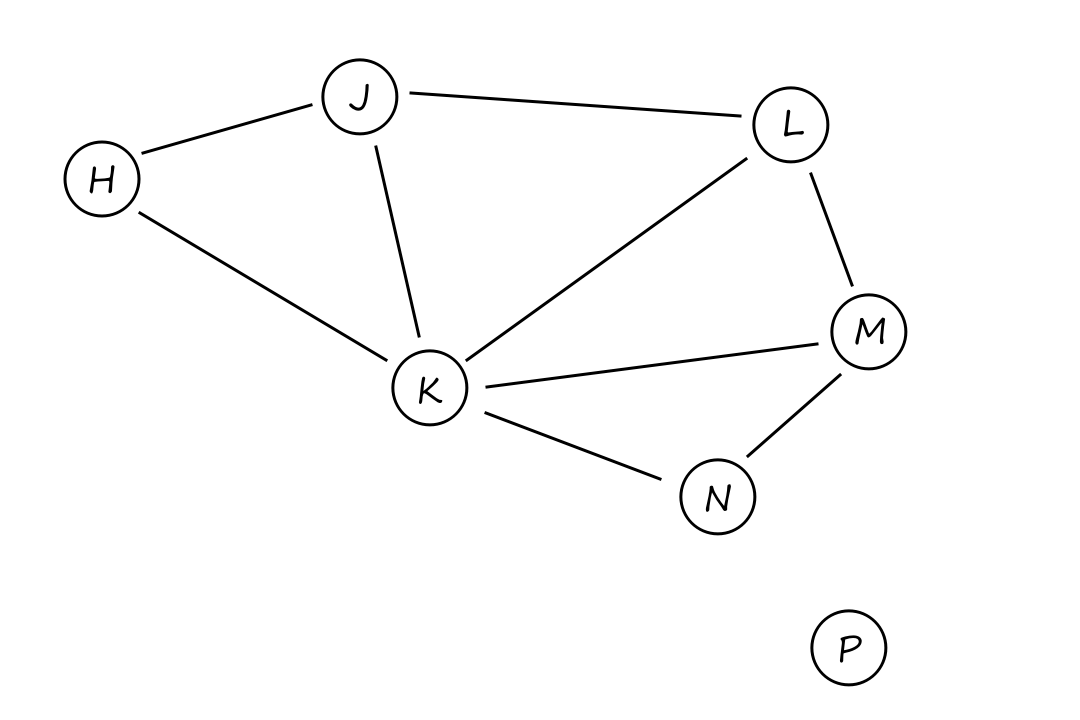
To spare myself the trouble of actually drawing a map, I'll represent a region as a node instead. `P` is a little island all on its own.
This is actually called a constraint graph, where the edges connect variables that are constrained.
We formally define our CSP as:
`chi={H,J,K,L,M,N,P}`
`D_i={text(red), text(green), text(blue)}`
`bbbC={K ne H, K ne J, K ne L, K ne M, K ne N, H ne J, J ne L, L ne M, M ne N}`
Because we're lazy, `K ne H` is a shortcut for `(:(K,H), K ne H:)=(:(K,H),{(text(red),text(green)),(text(red),text(blue)),(text(green),text(red)),(text(green),text(blue)),(text(blue),text(red)),(text(blue),text(green))}:)`.
One solution is `{H=text(red),J=text(green),K=text(blue),L=text(red),M=text(green),N=text(red),P=text(blue)}`.
While it may seem like adding constraints to a problem might make it harder to solve, it actually makes things a lot easier for our algorithms. By adding constraints, the number of possible states are reduced. For example, once we've decided that we want `K` to be blue, that eliminates all the states where `H`, `J`, `L`, `M`, and `N` are blue.
Without the constraint, there are `3^5=243` possible states to consider (`3` colors for each of the `5` regions).
With the constraint, there are only `2^5=32` possible states to consider (`2` colors for each of the `5` regions).
Constraint Propagation: Inference in CSPs
This idea of reducing the number of possible states is constraint propagation, which means using the constraints to reduce the number of valid values for a variable, which in turn can reduce the number of valid values for other variables.
Before we can begin searching for a solution, we need the graph to be consistent with the constraints. This is referred to as local consistency.
Node consistency
A unary constraint is a constraint that only affects one variable at a time. For example, `P ne text(green)`.
A variable is node-consistent if all the values in the variable's domain satisfy the variable's unary constraints. A graph is node-consistent if every variable is node-consistent.
Arc consistency
A binary constraint is a constraint that affects two variables at a time. `K ne H` is a binary constraint.
A variable is arc-consistent if all the values in the variable's domain satisfy the variable's binary constraints.
More specifically, a variable `X_i` is arc-consistent with `X_j` if for every value in the domain `D_i` there is some value in the domain `D_j` that satisfies the binary constraint on `X_i` and `X_j`.
The most popular algorithm for creating an arc-consistent graph is called AC-3. It essentially goes through each arc (edge) and tries to reduce the size of each variable's (node's) domain.
If all variables have a domain of size `1`, then the problem is solved. If there is any variable with a domain of size `0`, then there is no solution.
Path consistency
Path consistency makes sure three variables are consistent with each other. The name comes from the idea that the path between two variables is consistent with a third variable in the middle of the path.
A two-variable set `{X_i,X_j}` is path-consistent with respect to `X_m` if, for every assignment `{X_i=a,X_j=b}` (consistent with the constraints on `X_i` and `X_j`), there is an assignment to `X_m` that satisifes the constraints on `{X_i,X_m}` and `{X_m,X_j}`.
`K`-consistency
A CSP is `k`-consistent if, for any set of `k-1` consistent variables, a consistent value can be assigned to any `k^(th)` variable.
Node consistency is `1`-consistency. Arc consistency is `2`-consistency. Path consistency is `3`-consistency.
A CSP is strongly `k`-consistent if it is `k`-consistent, `(k-1)`-consistent, ..., `1`-consistent.
Global constraints
A global constraint is a constraint that affects any number of variables at a time. It doesn't need to, but a global constraint can affect all of the variables at a time. In fact, one of the most common constraints is that each variable must have a different value (this constraint is referred to as an "Alldiff" constraint).
A resource constraint is a constraint resulting from the limited number of resources available (this is sometimes referred to as an "Atmost" constraint). For example, suppose there are `4` tasks and only `10` people available to do them. If each task needs at least `3` people, then there is no solution.
For problems that deal with larger numbers of resources, limiting the range of values a variable can have is more appropriate. This is bounds propagation.
For example, suppose there are two airplanes where one can carry `165` people and the other can carry `385`. So the initial domains are
`D_1=[0,165]`
`D_2=[0,385]`
Let's say our constraint is that the two flights together must carry `420` people. Using bounds propagation, we now have the domains
`D_1=[35,165]`
`D_2=[255,385]`
A CSP is bounds-consistent if for every variable `X` (for both the lower-bound and upper-bound values of `X`), there exists some value for `Y` that satisifies the constraint between `X` and `Y` for every variable `Y`.
Backtracking Search for CSPs
After applying the constraints to a CSP, we then have to search for a solution (if applying the constraints didn't already give us a solution for free).
The basic idea behind backtracking search is that it repeatedly chooses an unassigned variable and tries different values in the domain of that variable. If a solution isn't found, the algorithm backtracks and tries again with different values. It's kinda like "Let's try this. Then let's try this. Then let's try this. Oops, that didn't work! Let's try this instead."
function BACKTRACKING-SEARCH(csp)
  return BACKTRACK(csp, {})
function BACKTRACK(csp, assignment)
  if assignment is complete then return assignment
  var = SELECT-UNASSIGNED-VARIABLE(csp, assignment)
  for each value in ORDER-DOMAIN-VALUES(csp, var, assignment) do
    if value is consistent with assignment then
      add {var = value} to assignment
      inferences = INFERENCE(csp, var, assignment)
      if inferences != failure then
        add inferences to csp
        result = BACKTRACK(csp, assignment)
        if result != failure then return result
        remove inferences from csp
      remove {var = value} from assignment
  return failure
INFERENCE() is a function that checks for consistency. ORDER-DOMAIN-VALUES() is a function that sorts the values in a way that we think is optimal.
For a CSP with `n` variables, each with a domain size of `d`, the search tree would have a depth of `n`.
At the top level, there are `n` nodes and each of them will have `d` children, so the branching factor is `nd` for the first level. At the second level, there are `n-1` nodes and each of them will have `d` children, so the branching factor is `(n-1)d` for the second level. This continues until the bottom where there is `1` node and `d` children.
So the tree has `n!d^n` leaves.
However, CSPs are commutative, meaning that the order that we assign the variables doesn't matter. For example
`{H=text(red),J=text(green),K=text(blue),L=text(red),M=text(green),N=text(red),P=text(blue)}`
is the same as
`{L=text(red),M=text(green),P=text(blue),H=text(red),J=text(green),N=text(red),K=text(blue)}`.
Since the order of the `n` variables doesn't matter for distinguishing solutions, we can divide by `n!` to remove repeated paths, resulting in the tree actually being `O(d^n)`.
Variable and value ordering

Going back to our map, let's say we arbitrarily start at `H` and arbitrarily choose red for it. Then we arbitrarily choose green for `J`. From these two decisions, we can see that `K` is now forced to be blue. This in turn, forces `L`, `M`, and `N` to be red, green, and red respectively.
If we had instead decided to pick a color for `L` before looking at `K`, we would not have had it this easy. In fact, if we had decided `L` to be blue, there would have been no valid value for `K` and we would have had to start over.
This highlights that when deciding which unassigned variable to look at next, we should look at the variable with the fewest valid values. This strategy is the minimum-remaining-values (MRV) heuristic. It is also called the "fail-first" heuristic because it picks a variable that is most likely to cause a failure, which allows the tree to be pruned. In our example, picking blue for `L` caused a failure, so all the possible map configurations where `L` is blue (and `H` is red and `J` is green) can be pruned away.
But notice how we were still making arbitrary decisions for the first two moves. The MRV heuristic isn't really helpful in the beginning because all the variables have the same number of valid values. So another heuristic that helps us pick a variable at the start is the degree heuristic. It selects the variable that is involved in the most constraints with other unassigned variables. In our map, `K` has a constraint with `5` other variables (i.e. it has degree `5`), so it should be picked first. It just so happens that starting with `K` guarantees that a solution will be found right away.
So we have heuristics for deciding which variable to look at first, but there is one more choice to think about and that is which value to assign first. Let's say we picked `H` to be red and `J` to be green, and we decided to look at `L` (despite knowing that looking at `K` first was better). We know that picking blue for `L` is not a good idea since it leaves no choices available for `K`, so we choose red instead.
Instead of picking a value that will cause a failure, we want to pick a value that will work. More specifically, we want to pick a value that will rule out the fewest choices for the neighboring variables, giving them as much flexibility as possible. This is the least-constraining-value heuristic.
Variable selection should be fail-first and value selection should be fail-last. This is because starting at the most restrictive variable reduces the number of times we have to backtrack. If we know a variable is going to cause failures, it doesn't make sense to start somewhere else and keep hitting that failure. It's better to just prevent that failure in the first place.
Value selection should be fail-last because we want to find a solution as soon as possible. We don't need to find all possible combinations of values that work; we just need to find one set of values that work.
Interleaving search and inference
As we saw before, inference (using AC-3) can reduce the size of a variable's domain before the search starts. But we can do this during the search as well by doing forward checking. Whenever a value is assigned to a variable, we look at the other variables involved in a constraint with this variable and remove inconsistent values from their domains.

Let's say we start with `H` red. Once we have this, we know that `K` and `J` can't be red, so we remove red from their domains.
Then we choose `L` green. Once we have this, we know that `J`, `K`, and `M` can't be green, so we remove green from their domains.
Then we choose `N` blue. Once we have this, we know that `K` and `M` can't be blue, so we remove blue from their domains.
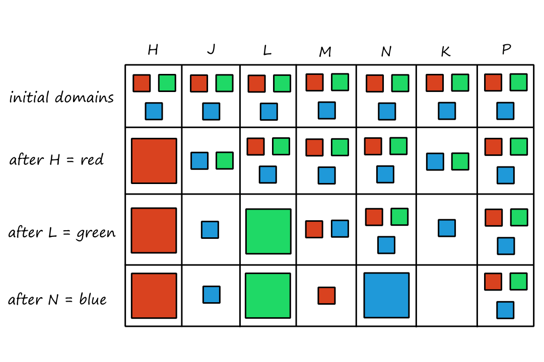
At this point, we can see that there are no valid values left for `K`. So we have to backtrack and try a different value for `N`.
Intelligent backtracking: Looking backward
Whenever an inconsistency is found, the backtracking algorithm goes up one level to the previous variable and tries a different value. This is called chronological backtracking because the most recent decision point is revisited.
This is simple, but it can be a little inefficient.
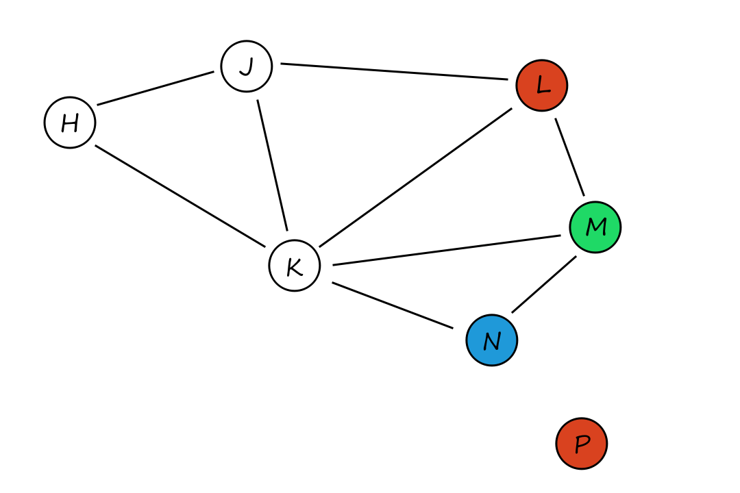
Let's say we started with `L` red, `M` green, `N` blue, and `P` red in that order. Now we see that there is no valid color for `K`, so we backtrack and consider a different value for `P`. Unfortunately, we can see that choosing a different value for `P` won't change anything since `P` wasn't causing the problem; we would have to backtrack one more level to `N`. But the algorithm will be inefficient and try different values of `P` until none of them work and then backtrack to `N`.
Since the set `{L=text(red),M=text(green),N=text(blue)}` was responsible for `K` not having any valid values, we call this set the conflict set for `K`. If we keep track of this set, we can backjump to the most recent assignment in the conflict set, which would be `N` in this case.
Forward checking prevents inconsistent situations from being reached in the first place. Doing both forward checking (or any consistency checking in general) and backjumping is redundant.
Constraint learning
If we reach an inconsistency, we can remember what the conflict set was that led to the inconsistency so we don't run into it again. This set is aptly called a no-good.
Local Search for CSPs
The local search algorithms we saw before can be used to solve CSPS. The idea is to assign a value to every variable at the beginning, even if they're inconsistent. Then we randomly choose a variable that is violating one or more constraints and change its value to something that violates fewer constraints. And we keep doing this until we find a solution. (Or keep going forever if there is no solution. 😏)
The min-conflicts heuristic chooses the value that results in the minimum number of violated constraints with other variables.
Summary of Chapter 6
- Constraint satisfaction problems (CSPs) represent a state with a set of variable/value pairs and represent the conditions for a solution by a set of constraints on the variables.
- Inference techniques use the constraints to rule out certain variable assignments. Some of the inference techniques are node, arc, path, and `k`-consistency.
- Backtracking search is a form of depth-first search that is commonly used to solve CSPs.
- The minimum-remaining-values and degree heuristics are domain-independent methods for deciding which variable to choose next in a backtracking search.
- The least-constraining-value heuristic helps in deciding which value to try first for a variable.
- Conflict-directed backjumping backtracks directly to the source of the problem.
- Constraint learning records the conflicts as they are encountered during search in order to avoid the same conflict later on.
- Local search using the min-conflicts heuristic is good.
Now, we'll look at multi-agent environments. In particular, competitive environments where two or more agents have conflicting goals. Problems in these environments are called adversarial search problems.
Game Theory
Apparently, chess, Go, and poker are popular games to study in the AI community.
Two-player zero-sum games
Game theorists call these types of games deterministic, two-player, turn-taking, perfect information, zero-sum games. "Perfect information" means "fully observable" and "zero-sum" means that what is good for one player is just as bad for the other. A move is an "action" and a position is a "state".
A game can be formally defined by specifying:
- the initial state, which describes how the game is set up at the start
- `S_0`
- the player whose turn it is to move in state `s`
- `text(TO-MOVE)(s)`
- the set of legal moves in state `s`
- `text(ACTIONS)(s)`
- the transition model, which defines the state resulting from taking action `a` in state `s`
- `text(RESULT)(s,a)`
- a terminal test, which is true when the game is over
- states where the game has ended are called terminal states
- `text(IS-TERMINAL)(s)`
- a utility function, which assigns numerical values to the outcome of the game
- in chess, a win is `1`, a loss is `0`, and a draw is `1/2`
- `text(UTILITY)(s,p)`
Chess is considered a "zero-sum" game even though the sum of the outcomes is `1`. However, if we imagine that each player "paid `1/2`" to play, then the winner wins `1/2` and the loser loses `1/2`.
Instead of using a search tree like the one we saw earlier, we'll be using a game tree, which takes into account that there are multiple players. And speaking of players, we'll be calling our two players MAX and MIN.
Here's an example of a (partial) game tree for tic-tac-toe:
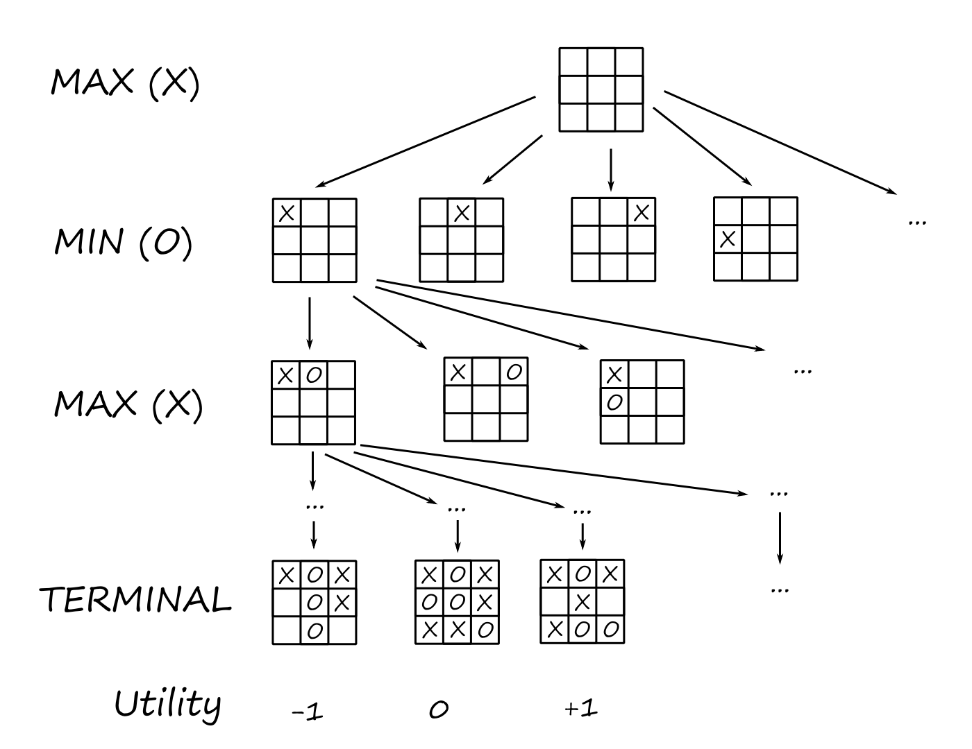
Optimal Decisions in Games
Since each player is responding to each other's moves, the strategy for both players is a conditional plan (if that player does this, I'll do this).
In games that have a binary outcome (e.g., win or lose), we could use AND-OR search to generate the conditional plan. For games with multiple outcomes, we need something a little more general.
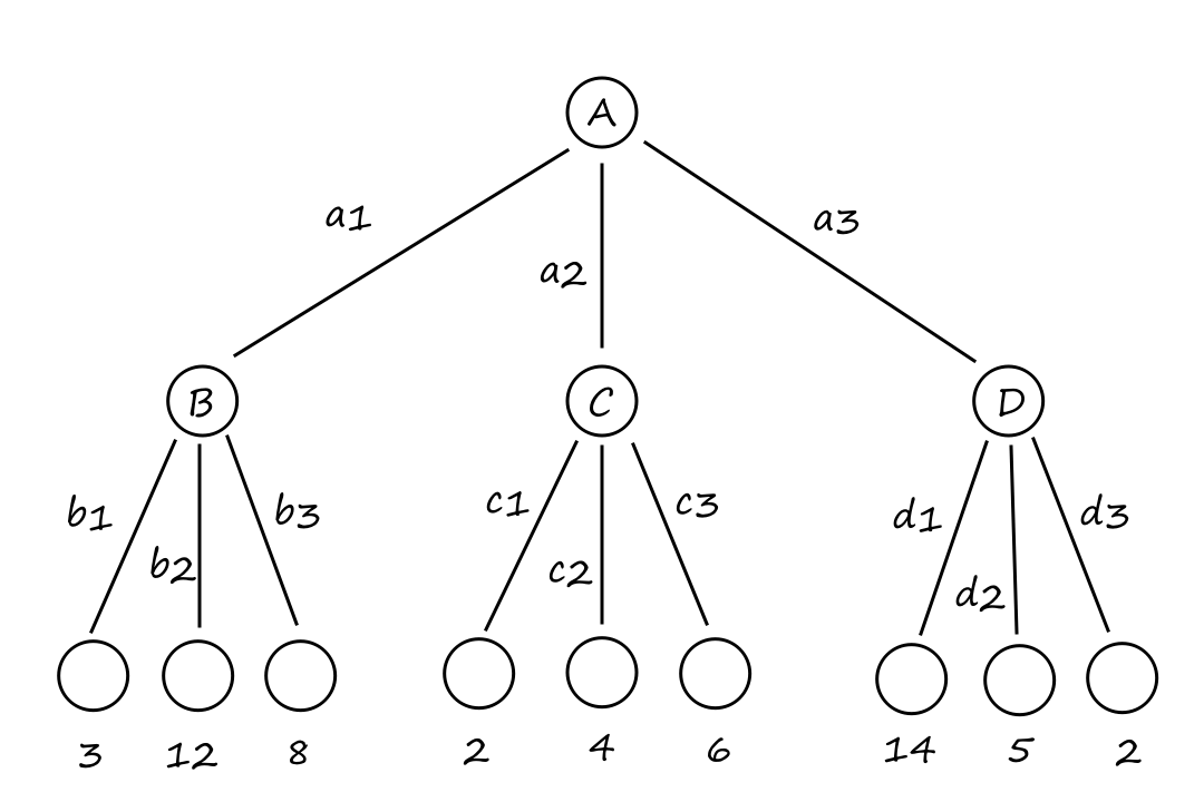
Consider the simple game above where MAX is trying to reach one of the bottom-row nodes with the highest value and MIN is trying to have MAX end up at the node with the lowest value (depending on MAX's first move). MAX moves first and gets to pick a path `a_1`, `a_2`, or `a_3`. Then it is MIN's turn to decide which bottom-row node MAX ends up at.
For example, MAX might want to reach the node with `14`, so MAX will choose `a_3`. At this point, MIN has three options `d_1`, `d_2`, `d_3`. Since MIN wants MAX to have the lowest score possible, MIN will choose `d_3`, so MAX will end up with a score of `2`.
That strategy didn't really go so well for MAX, so let's look at another one. This time, MAX wants `12`, so MAX will choose `a_1`. MIN will then choose `b_1` so that MAX ends up with `3`, the lowest out of the three choices.
We can see that `3` is the highest score MAX can hope to get if MIN plays optimally. And if you took the time to verify that, then you'll notice that you played the game backwards (starting from the bottom and moving up) to check.
This is essentially the idea behind the minimax search algorithm.
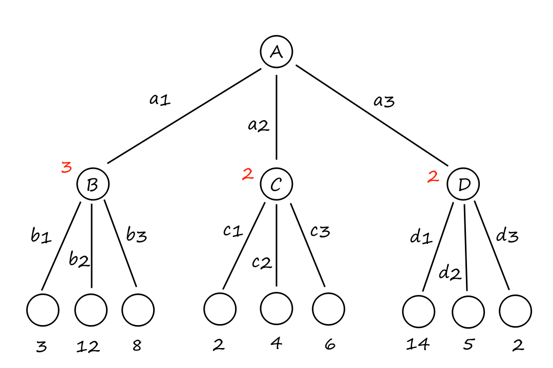
`B` has a minimax value of `3` because if MAX chooses `a_1`, the highest score MAX can get is `3` if MIN plays optimally.
Each node is assigned a minimax value that represents how "good" that position/move is for a player, assuming the other player plays optimally. In this game, MAX wants to choose the node with the maximum minimax value and MIN wants to choose the node with the minimum minimax value.
The minimax value of the terminal nodes are just the values defined by the game's `text(UTILITY)` function (for terminal nodes, their utility is the score we get when the game ends). Then the minimax values are propagated up the game tree using the same reasoning we used to analyze the game above.
The minimax search algorithm
This is a recursive search algorithm that goes all the way down to the leaves and then backs up the minimax values up the tree as the recursion unwinds.
function MINIMAX-SEARCH(game, state)
  player = game.TO-MOVE(state)
  value, move = MAX-VALUE(game, state)
  return move
function MAX-VALUE(game, state)
  if game.IS-TERMINAL(state) then return game.UTILITY(state, player), null
  v = -infinity
  for each a in game.ACTIONS(state) do
    v2, a2 = MIN-VALUE(game, game.RESULT(state, a))
    if v2 > v then
      v, move = v2, a
  return v, move
function MIN-VALUE(game, state)
  if game.IS-TERMINAL(state) then return game.UTILITY(state, player), null
  v = infinity
  for each a in game.ACTIONS(state) do
    v2, a2 = MAX-VALUE(game, game.RESULT(state, a))
    if v2 < v then
      v, move = v2, a
  return v, move
Let `m` be the maximum depth of the tree and assume there are `b` legal moves at each point.
The time complexity of minimax search is `O(b^m)` and the space complexity is `O(bm)` (the reasoning for the space complexity is the same as the reasoning for the space complexity of depth-first search; this is a depth-first algorithm after all).
Optimal decisions in multiplayer games
To create game trees for games with more than two players, we assign a group of values (one value for each player) to each node. Consider a game (similar to the one before) where all players are trying to get to the node that will give them (individually) the highest score possible.
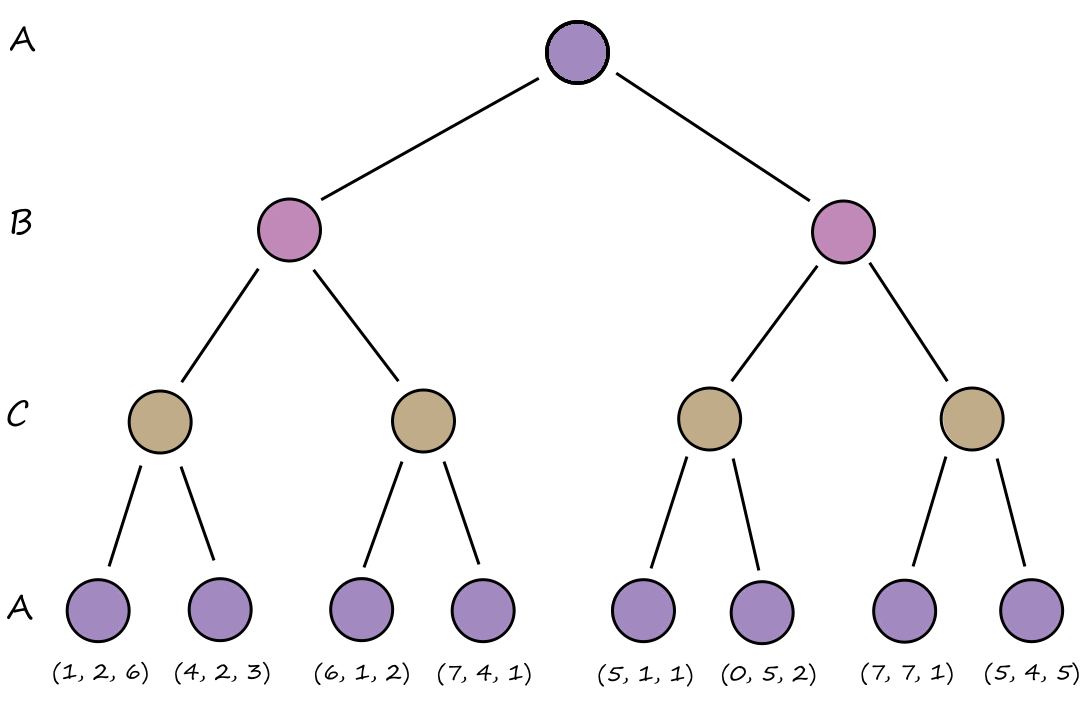
Let's say we have three players `A`, `B`, and `C`. So each node will have a group of minimax values `(a,b,c)` where `a` is the minimax value for `A`, `b` is the minimax value for `B`, and `c` is the minimax value for `C`. `A` is trying to get to the node with the highest `a` value, `B` is trying to get to the node with the highest `b` value, and `C` is trying to get to the node with the highest `c` value.
Suppose `A` wants to get to the node `(7,4,1)`, so `A` moves left. At this point, `B` would also want to get to the node `(7,4,1)`, so `B` moves right. From the remaining options, `C` wants to get to the node `(6,1,2)`, so `C` moves left. So the final score for all three players is `A:6`, `B:1`, `C:2`.
This is the game tree assuming everyone plays optimally:
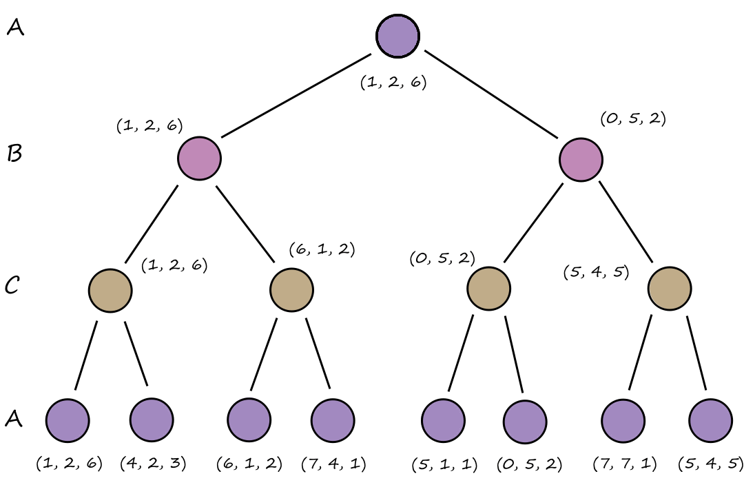
`A`'s best move is left since the minimax value of the left node `(1)` is greater than the minimax value of the right node `(0)`.
Again, the terminal nodes have their minimax values defined by the game's `text(UTILITY)` function, and the values are passed up the tree depending on which player's turn it is.
Alpha-Beta Pruning
We can actually sometimes deduce the minimax value of a node without having to fully expand it. This means that we can optimize the algorithm by not examining all the nodes. If we can deduce that it is not optimal for a player to go down a certain path, we can skip it, which resultingly prunes the tree.
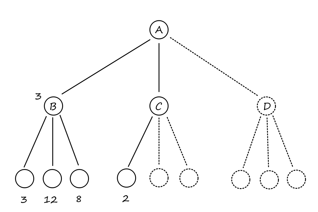
Suppose we're running the algorithm and we've already discovered the minimax value of `B`. And now when we're calculating the minimax value of `C`, we find that its first child has a value of `2`. We don't need to look at the minimax values of the other two children because the minimax value of `C` will be at most `2`. If the other two children have minimax values higher than `2`, then MIN will move to the node with minimax value `2`. If the other two children have minimax values lower than `2`, then MIN will move to those nodes, making MAX's score even lower. No matter what those two children of `C` are, it's not in MAX's best interest to move to `C` because moving to `B` is a better option.
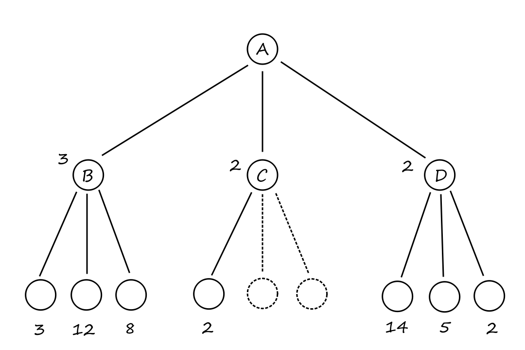
We do however, need to explore all of `D`'s children though. The minimax values of the first two children are `14` and `5`, both of which are higher than `3`, so MAX would still want to go down this path. It's not until we look at the last child that we can determine that this path is not optimal for MAX.
`text(MINIMAX)(text(root)) = max(min(3,12,8),min(2,x,y),min(14,5,2))`
`= max(3,min(2,x,y),2)`
`= max(3,z,2)` where `z = min(2,x,y) le 2`
`=3`
It is called alpha-beta pruning because `alpha` and `beta` are used as bounds to determine whether a part of the tree can be pruned. `alpha` is the highest minimax value found so far and `beta` is the lowest minimax value found so far.
function ALPHA-BETA-SEARCH(game, state)
  player = game.TO-MOVE(state)
  value, move = MAX-VALUE(game, state, -infinity, infinity)
  return move
function MAX-VALUE(game, state, α, β)
  if game.IS-TERMINAL(state) then return game.UTILITY(state, player), null
  v = -infinity
  for each a in game.ACTIONS(state) do
    v2, a2 = MIN-VALUE(game, game.RESULT(state, a), α, β)
    if v2 > v then
      v, move = v2, a
      α = MAX(α, v)
    if v ≥ β then return v, move
  return v, move
function MIN-VALUE(game, state, α, β)
  if game.IS-TERMINAL(state) then return game.UTILITY(state, player), null
  v = infinity
  for each a in game.ACTIONS(state) do
    v2, a2 = MAX-VALUE(game, game.RESULT(state, a), α, β)
    if v2 < v then
      v, move = v2, a
      β = MIN(β, v)
    if v ≤ α then return v, move
  return v, move
Notice that if v ≤ α then return v, move is the reasoning we used to stop exploring `C`. `alpha` is `3` (the highest value we've seen so far) and `v` is `2`. Since `2 le 3`, we're gonna return `2`, i.e., we're assigning the minimax value of `C` to `2`.
Move ordering
Notice that if the last child of `D` (the one with minimax value `2`) had been generated first, then we could've pruned `D`'s other children. This means that, if possible, we should try to examine successors that allow us to prune the tree.
A move that prunes a tree when examined is called a killer move. Examining those moves first is called the killer move heuristic. It's not examining the node and then finding out that it prunes the tree; it's knowing ahead of time that examining that node will prune the tree. This information comes from past experience. Maybe we have a collection of winning moves and we find a move at our current state in that collection.
In the best case, alpha-beta would only need to examine `O(b^(m//2))` nodes, compared to minimax's best case of `O(b^m)`. When we prune a tree, we're kinda removing half of it.
Heuristic Alpha-Beta Tree Search
Even with alpha-beta pruning and good move ordering, there are still too many states to explore for games like chess. One way to deal with this is to use a Type A strategy, which considers all possible moves until a certain depth. Then it uses a heuristic function to estimate the utility of the rest of the states.
A Type A strategy searches a wide but shallow part of the tree. Because of this, a Type A strategy is not good for games with large branching factors, like Go.
A Type B strategy ignores moves that look bad and only searches moves that look promising. This results in searching a deep but narrow part of the tree.
There's a cutoff test to determine when to stop searching and start estimating. This effectively treats nonterminal nodes as if they were terminal nodes.
Evaluation functions
A heuristic evaluation function gives us an estimate of a state's expected utility.
`text(EVAL)(s,p)=text(UTILITY)(s,p)` for terminal states.
`text(UTILITY)(text(loss),p) le text(EVAL)(s,p) le text(UTILITY)(text(win),p)` for nonterminal states.
Evaluation functions work by calculating various features of the state. The information from those features is used to assign a numerical value to that state. A good evaluation function should not take too long to compute (obviously). More importantly, the evaluation function should be strongly correlated with the actual chances of winning.
For example, one feature we could use is the number of pieces that each player (white vs black) has remaining. If there's a move that results in white having more pieces, then that state should have a high evaluation function value for white.
Of course, simply having more pieces doesn't necessarily mean it's better. It depends on what types of pieces they are. For example, a queen is much more valuable than having eight pawns and no queen. We take things like this into account by adding weight to certain features that are more important than other features.
Mathematically, this kind of evaluation function is called a weighted linear function.
`text(EVAL)(s) = w_1f_1(s)+w_2f_2(s)+...+w_nf_n(s)`
where each `f_i` is a feature, such as "number of white bishops"
However, using a linear function only works when the features are independent of each other, which isn't the case in chess. Bishops are generally worth more when there are fewer pieces in the game, i.e., number of bishops and number of pieces remaining are not independent.
Cutting off search
To implement this, we can modify ALPHA-BETA-SEARCH by replacing
if game.IS-TERMINAL(state) then return game.UTILITY(state, player), null
with
if game.IS-CUTOFF(state, depth) then return game.EVAL(state, player), null
Using an evaluation function that just counts the number of pieces is very simple and can lead to errors. For example, suppose the algorithm stops at the cutoff and finds a state where black has more pieces than white, so black moves to that state. But then white moves to capture black's queen! If the algorithm had been able to look ahead, then it would've known that it was not a favorable position after all.
Positions where a pending move can wildly swing the evaluation are called nonquiescent positions. The evaluation function should be used only for quiescent positions, and search should continue until quiescent positions are reached.
Forward pruning
Alpha-beta pruning prunes parts of the tree that were for sure bad moves. Forward pruning prunes parts of the tree that look like they have bad moves.
Forward pruning is a Type B strategy.
One way to implement forward pruning is to use beam search, which considers a "beam" of `n` moves. Of course, there's a chance that we miss the the best move by doing this.
Monte Carlo Tree Search
Monte Carlo tree search (MCTS) goes through many simulations to determine which moves are good. Basically, the algorithm plays out many games of "what if I do this and what if they do this?" and sees which choices led to wins and losses. So instead of using a heuristic evaluation function to assign values to states, it uses an average utility score (defined by the number of wins/losses and games) to assign values to states.
A pure Monte Carlo search does `N` simulations from the current state of the game and keeps track of which moves (from the current position) has the highest win percentage.
While it's not possible to know exactly how an opponent is going to respond to a move in a simulation, there are almost always certain moves that are better than others, and we can create playout policies that tell the algorithm what these moves are so they can prioritize those moves in the simulations.
Let's suppose we have this tree for a game played by pink and brown. Each fraction in the node is the number of simulations won over the number of simulations played. Our current state is the pink `37//100`, so from here, there are `3` possible moves we can consider. One move won `60` out of the `79` simulations; the second move won `1` out of `10` simluations; and the third move won `2` out of `11` simulations.
It makes sense to choose the move that had the highest win percentage, but this doesn't necessarily mean the other two moves are bad. This is because we only had `10` and `11` simluations for those moves; it's possible that they could have performed even better if more simluations had been played out.
Likewise, the move with the highest win percentage doesn't always mean it's the best move to make either. Winning `2` out of `3` simulations isn't enough information to know if the move is actually good or not.
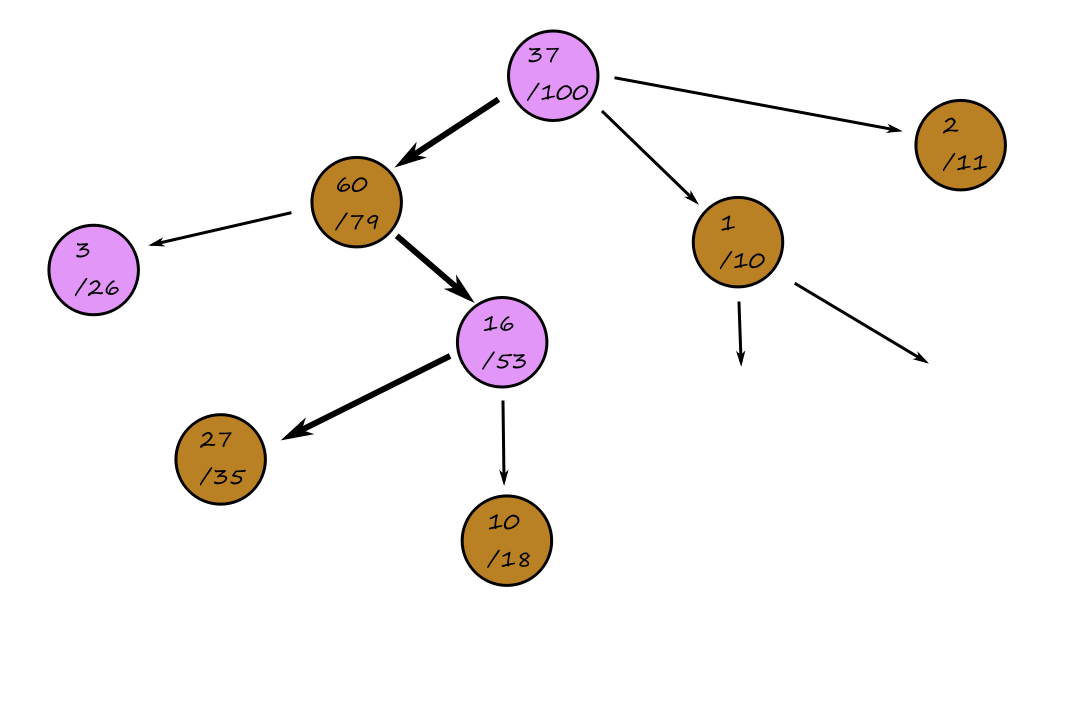
This decision about which state to go to next is decided by a selection policy, i.e., the selection policy tells the algorithm which state to go to next. There are two factors that influence the selection policy: exploitation and exploration. Exploitation is choosing states that have performed well (e.g., choosing the move with the highest win percentage) and exploration is choosing states that have had only a few simulations (to gather more information and to take a chance on it turning out to be a good move).
So now the search has progressed three moves later and our current state is at the brown `27//35`. It's time to run a simulation. (The moves that are played in this simulation are decided by the playout policy.)
Let's say that the simulation resulted in a loss for pink. Now we have to update the tree with this new information. This step is called back-propagation.

To summarize the process:
- Selection: keep choosing moves (guided by the selection policy) until we reach a leaf
- Expansion: generate a new child
- Simulation: play out a simulation (guided by the playout policy)
- Back-propagation: update all the search tree nodes with the new information
One very effective selection policy is called "upper confidence bounds applied to trees" (UCT). It uses a formula (UCB1) to rank each possible move.
`text(UCB1)(n)=(U(n))/(N(n))+C*sqrt((logN(text(PARENT)(n)))/(N(n)))`
`U(n)` is the total utility (e.g., number of wins) of all simulations that went through node `n`.
`N(n)` is the number of simulations through node `n`.
I think `text(PARENT)(n)` is the number of times `n`'s parent node has been selected for exploration.
`C` is a constant that balances exploration and exploitation.
`(U(n))/(N(n))` is the exploitation term and `sqrt((logN(text(PARENT)(n)))/(N(n)))` is the exploration term.
Stochastic Games
Stochastic games are ones that involve randomness and luck. Like games that involve rolling dice. In backgammon, the possible moves that a player can make is determined by the result of the dice rolls. So we can't really build the game tree the same way we did before because we don't know what the possible moves will be.
We have to include chance nodes, which represent a possible outcome from the random aspect of the game. So if a die can have `6` different values, then there will be `6` chance nodes for each value of the die and then we list all the possible moves for each chance node. If we're rolling two dice, then there will be a chance node for every possible pair of values.
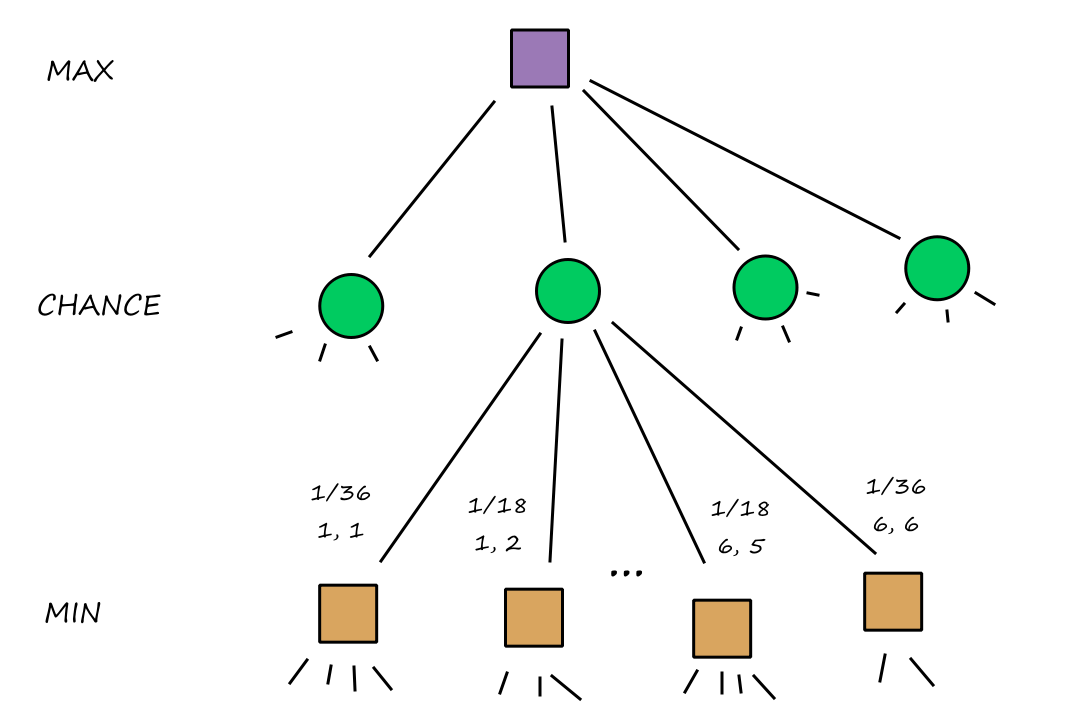
For a chance node, there is a branch for each possible outcome of rolling two dice. The probability of rolling a `1` and a `1` is `1/36`. The probability of rolling a `1` and a `2` is `1/18`.
Since we don't know for sure that a chance node will be reached, they don't have definite minimax values. Instead, each chance node has an expectiminimax value, which is the sum of the minimax values of each action weighted by the probability of that action (this is the expected value of the chance node).
The expectiminimax value of a non-chance node is its minimax value.
Evaluation functions for games of chance
Recall that in heuristic alpha-beta search, we kept searching until a certain point, then used a heuristic function to estimate the rest of the minimax values. For stochastic games, we can do the same, but we need a slightly different heuristic function.
Let's go back to the game where MAX is trying to reach the node with the highest value and MIN is trying to have MAX end up at the node with the lowest value. Suppose we have this game tree:
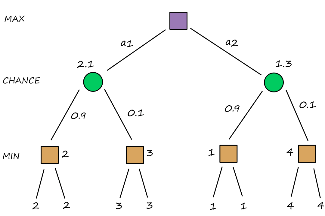
The left chance node's expectiminimax value is `2*0.9+3*0.1=2.1`.
We can see that the left chance node has a higher expectiminimax value, so MAX should go left (move `a_1`). We can also see that this is the optimal move for MAX since moving right means that there is a `90%` chance that MIN will be able to go to the node with `1`.
But let's look at what happens if the heuristic function had assigned different values to each of the nodes at the cutoff point.
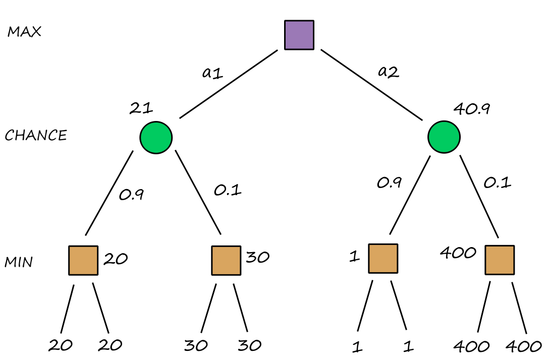
Now, the right chance node has a higher expectiminimax value, so MAX will go right (move `a_2`). But we can see that this is not the optimal choice because there is a `90%` chance that MIN will be able to go to the node with `1`.
From this, we can see that the heuristic function must also take into account the probabilities when calculating the utility. (I might go into more detail on this? Let's see where the class goes.)
Partially Observable Games
Kriegspiel: Partially observable chess
Kriegspiel is an interesting version of chess where each player has their own board, and each player's board has only their own pieces. Each player proposes a move and a referee (who can see both players' boards) tells them if the move is legal or illegal. If the move is illegal, that player keeps proposing moves until a legal one is found. If the move is legal, the referee announces captures, checks, and mates if any of those happened.
Using belief states helps here. In the context of games, a belief state is the set of all board states that are logically possible based on the moves that have happened so far. With this, we can use the AND-OR search algorithm we saw before.
Instead of branches for each possible move the opponent might make, we have branches for every possible percept sequence that might be received.
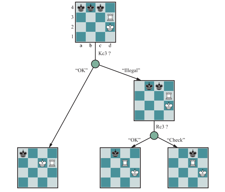
(I'm including a picture from the textbook because this is too complicated to draw myself. 😅)
While it's important to move pieces to the right places, playing optimally can be predictable, giving the opponent information. Sometimes, making random moves is optimal because it introduces an element of unpredictability that the opponent may not be prepared for.
Summary of Chapter 5
- A game can be defined by the initial state (how the board is set up), the legal actions in each state, the result of each action, a terminal test (which says when the game is over), and a utility function that applies to terminal states to say who won and what the final score is.
- In two-player, discrete, deterministic, turn-taking zero-sum games with perfect information, the minimax algorithm can select optimal moves by a depth-first enumeration of the game tree.
- The alpha-beta search algorithm computes the same optimal move as minimax, but achieves much greater efficiency by eliminating subtrees that are provably irrelevant.
- Usually, it is not possible to consider the whole game tree (even with alpha-beta), so we need to cut the search off at some point and apply a heuristic evaluation function that estimates the utility of a state.
- An alternative called Monte Carlo tree search (MCTS) evaluates states not by applying a heuristic function, but by playing out the game all the way to the end and using the rules of the game to see who won. Since the moves during the playout may not have been optimal moves, the process is repeated multiple times and the evaluation is the average of the results.
- Many game programs precompute tables of best moves in the opening and endgame so that they can look up a move rather than search for one.
- Games of chance can be handled by expectiminimax, an extension to the minimax algorithm that evaluates a chance node by taking the average utility of all its children, weighted by the probability of each child.
- In games of imperfect information, like poker, optimal play requires reasoning about the current and future belief states of each player. A simple approximation can be obtained by averaging the value of an action over each possible configuration of missing information.
Knowledge-Based Agents
So far, all we've seen are problem-solving agents. As powerful as they are, they aren't able to reason or adapt to new information.
Knowledge-based agents are able to use logic to make decisions. They have a knowledge base of sentences, which are the facts that are known by the agent. They use the sentences in their knowledge base to come up with new sentences (conclusions). This process is called inference.
The Wumpus World
Here, we'll go over an example of how a knowledge-based agent works.
The wumpus world is a cave with a monster (wumpus), a pile of gold, and a bunch of bottomless pits. The goal of the agent is to find the gold while avoiding the pits and the wumpus. The wumpus can be killed with an arrow, but the agent has only one arrow to use.
The wumpus world is partially observable, single-agent, deterministic, sequential, static, and discrete.
PEAS description:
- Performance measure: `+1000` for escaping with the gold, `-1000` for falling into a pit or being eaten by the wumpus, `-1` for each action taken, `-10` for using an arrow
- Environment: A `n xx n` grid of rooms. The locations of the gold and the wumpus are chosen randomly. Each square (other than the start) can be a pit with some probability (say `0.2`)
- Actuators: the agent can move forward, turn left, turn right, grab the gold, shoot an arrow, and climb out of the cave
- Sensors: the agent can perceive a stench (from the wumpus), a breeze (from a pit), a glitter (from the gold), a bump (when walking into a wall), and a scream (when the wumpus is killed)
- the stench and a breeze are detected when the agent is on a square next to a wumpus or a pit
Let's say our agent (denoted as `A`) starts in the lower-left corner. It doesn't detect a stench or a breeze so the two squares next to it are safe.
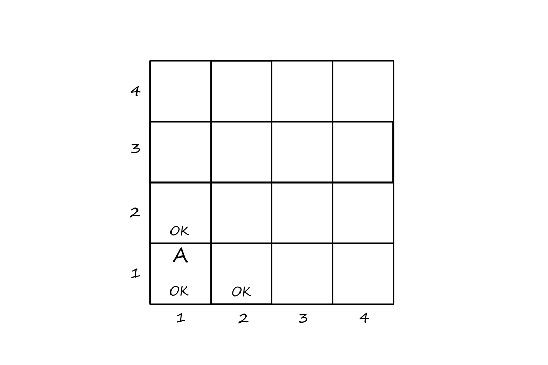
After moving right, the agent detects a breeze. The breeze could be coming from the square above or from the right. (Bear with me here, the agent can't lick its finger to see which direction the breeze is blowing.) There is only one square that is for sure safe, so the agent decides to go back and move there.
Here, the agent detects a stench. Theoretically, the stench could be coming from the square above or from the right. But since the agent didn't detect a stench in the previous state (image above), it knows the wumpus can't be in the square to the right.
Also, since the agent is not detecting a breeze, that means the square to the right is not a pit.
Avoiding the wumpus, the agent finds the gold!
Logic
In order for a knowledge-based agent to be able to reason and make inferences, it needs to understand logic.
A sentence has a truth value, i.e., it can either be true or false. Its truth value depends on the world (model) it's in.
The sentence `x+y=4` is true in a world where `x=2,y=2` and false in a world where `x=1,y=1`.
If a sentence `alpha` is true in model `m`, then `m` satisfies `alpha` (or `m` is a model of `alpha`).
The truth value of a sentence can depend on the truth value of another one. We say that a sentence can follow logically from another sentence.
The sentence `x=0` entails the sentence `xy=0`, i.e., the sentence `xy=0` follows logically from `x=0`.
`alpha` entails `beta` is denoted as `alpha |== beta`.
The formal definition of entailment is: `alpha |== beta` if and only if, in every model in which `alpha` is true, `beta` is also true.
`alpha |== beta iff M(alpha) sube M(beta)`
(`M(alpha)` is the set of models where `alpha` is true.)
Let's see how this can be applied to the wumpus world. Suppose the agent is at `[2,1]` (the second step when it detected a breeze).

`KB` is the agent's knowledge base. There are three possible models based on the knowledge that it feels a breeze on its current square (either the pit is in the square above, to the right, or both).
Let `alpha_1` be the sentence, "There is no pit in `[1,2]`." There are four possible models based on this sentence.
Notice that in every model in which `KB` is true, `alpha_1` is also true. That is, if you pick any model in `KB` and say "There is no pit in `[1,2]`", the sentence is true. This means that `KB` entails `alpha_1`, and the agent can conclude that there is no pit in `[1,2]`.
Now let `alpha_2` be the sentence, "There is no pit in `[2,2]`."
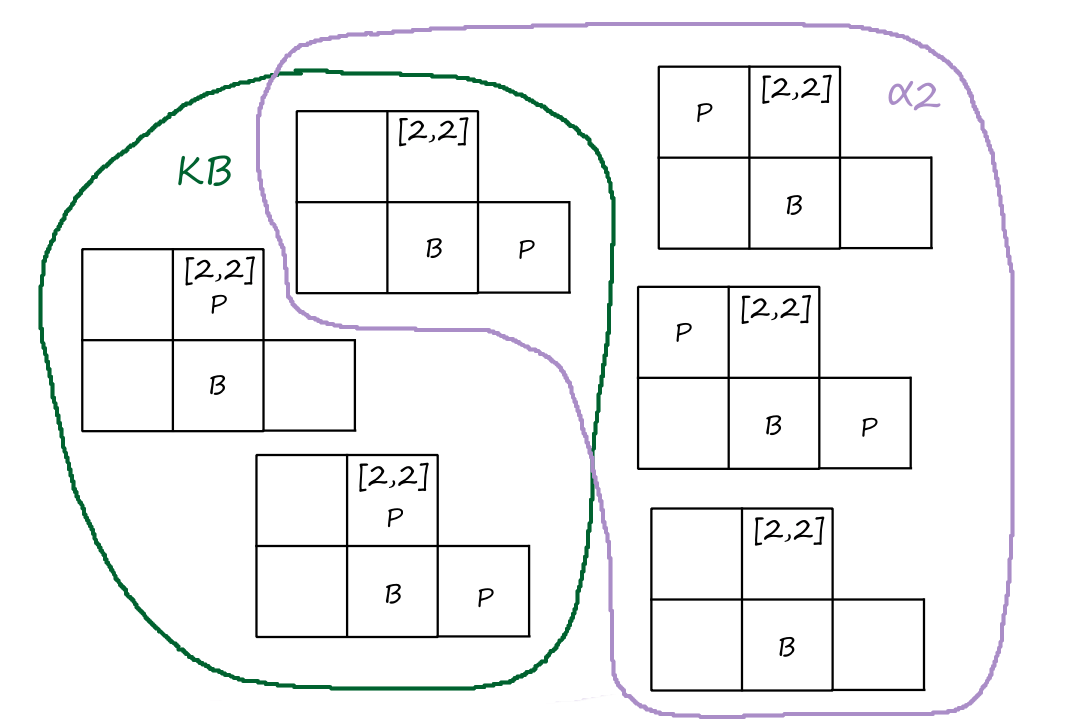
There are some models in `KB` where if we say "There is no pit in `[2,2]`", the sentence is false. So `KB` does not entail `alpha_2`, meaning that the agent cannot conclude that there is no pit in `[2,2]`.
Whether you realized it or not, we were running an algorithm to check entailment. The inference algorithm is called model checking.
An inference algorithm is sound or truth-preserving if it derives only entailed sentences. That is, the results of running the algorithm are all sentences that follow logically. An unsound algorithm makes things up.
If it's provable, it's true.
An inference algorithm is complete if it can derive any sentence that is entailed. That is, all sentences that follow logically can be derived using the algorithm.
If it's true, it's provable.
Propositional Logic: A Very Simple Logic
Syntax
A proposition is a sentence (that can be true or false). We use a symbol (typically a letter) to represent a proposition. For example, `W_(1,3)` can be the symbol for "there is a wumpus at `[1,3]`" and `P_(3,1)` can be the symbol for "there is a pit at `[3,1]`."
We can use logical connectives to turn sentences into complex sentences. The most common connectives are
- `not` (not). `not W_(1,3)` (the negation of `W_(1,3)`) means "there is no wumpus at `[1,3]`."
- `^^` (and). `W_(1,3) ^^ P_(3,1)` means "there is a wumpus at `[1,3]` and there is a pit at `[3,1]`."
- a sentence of this form is called a conjunction
- `vv` (or). `W_(1,3) vv P_(3,1)` means "there is a wumpus at `[1,3]` or there is a pit at `[3,1]`."
- a sentence of this form is called a disjunction
- `implies` (implies). `W_(1,3) implies not W_(2,2)` means "if there is a wumpus at `[1,3]`, then there is no wumpus at `[2,2]`."
- a sentence of this form is called an implication
- `iff` (if and only if). `W_(1,3) iff not W_(2,2)` means "there is a wumpus at `[1,3]` if and only if there is no wumpus at `[2,2]`."
- a sentence of this form is called a biconditional
An atomic sentence is a sentence without any connectives; it's just a single symbol.
A literal is an atomic sentence.
Complementary literals are literals where one is the negation of the other.
A clause is a disjunction of literals.
Semantics
The semantics of propositional logic defines the rules for determining the truth of a sentence. Here's a truth table that defines the connectives:
| `P` | `Q` | `not P` | `P^^Q` | `PvvQ` | `P implies Q` | `P iff Q` |
| false | false | true | false | false | true | true |
| false | true | true | false | true | true | false |
| true | false | false | false | true | false | false |
| true | true | false | true | true | true | true |
A simple knowledge base
Using all of this, we can build a knowledge base for the wumpus world. For the symbols, we have:
- `P_(x,y)` is true if there is a pit in `[x,y]`
- `W_(x,y)` is true if there is a wumpus in `[x,y]`
- `B_(x,y)` is true if there is a breeze in `[x,y]`
- `S_(x,y)` is true if there is a stench in `[x,y]`
- `L_(x,y)` is true if the agent is in `[x,y]`
With these symbols, we can create sentences that describe what the agent saw (and knows) in the wumpus world. (Each sentence will be labeled with `R_i`. The `R_i`s themselves are not symbols.)
- There is no pit in `[1,1]`
- `R_1`: `not P_(1,1)`
- A square is breezy if and only if there is a pit in a neighboring square
- `R_2`: `B_(1,1) iff (P_(1,2) vv P_(2,1))`
- `R_3`: `B_(2,1) iff (P_(1,1) vv P_(2,2) vv P_(3,1))`
- There is no breeze in `[1,1]`
- `R_4`: `not B_(1,1)`
- There is a breeze in `[2,1]`
- `R_5`: `B_(2,1)`
A simple inference procedure
We can now perform the model-checking algorithm a little more formally. The relevant symbols are `B_(1,1),B_(2,1),P_(1,1),P_(1,2),P_(2,1),P_(2,2),P_(3,1)`. A model is an assignment of true or false to each symbol.

Notice that in all the models in `KB`, statements `R_1,R_2,R_3,R_4,R_5` are all true. `KB` is true if `R_1` through `R_5` are true because those statements make up the knowledge base.
In fact, a systematic way to generate all the models in the knowledge base is to consider all the possible assignments to each symbol that make `R_1` through `R_5` true.
For example, here are the assignments for each of the three models in `KB` from top to bottom:
- `B_(1,1)=F,B_(2,1)=T,P_(1,1)=F,P_(1,2)=F,P_(2,1)=F,P_(2,2)=F,P_(3,1)=T`
- `B_(1,1)=F,B_(2,1)=T,P_(1,1)=F,P_(1,2)=F,P_(2,1)=F,P_(2,2)=T,P_(3,1)=F`
- `B_(1,1)=F,B_(2,1)=T,P_(1,1)=F,P_(1,2)=F,P_(2,1)=F,P_(2,2)=T,P_(3,1)=T`
Can `not P_(1,2)` (there is no pit in `[1,2]`) be derived from `KB`? Well, in all three models, `P_(1,2)` is false, meaning there is no pit in `[1,2]`. So yes, `not P_(1,2)` is entailed by `KB`.
Propositional Theorem Proving
If there are a lot of models in the knowledge base, then it's not efficient to check each model to determine entailment.
Theorem proving is a method of deriving a sentence by applying the rules of inference to the sentences in the knowledge base.
Two sentences are logically equivalent if they are true in the same set of models. This is denoted as `alpha -= beta`.
Two sentences are logically equivalent if and only if each of them entails the other:
`alpha -= beta` if and only if `alpha |== beta` and `beta |== alpha`
The deduction theorem says `alpha |== beta` if and only if the sentence `alpha implies beta` is true in all* models. This means we can decide if `alpha |== beta` by checking that `alpha implies beta` is true in every model.
*A sentence that is true in all models is valid. Valid sentences are also called tautologies. `P vv not P` is an example.
It might seem that `-=` and `iff` are the same. The subtle difference between them is that `-=` is used to make claims about sentences while `iff` is used to make sentences.
A sentence is satisfiable if it is true in at least one model.
One way of proving `alpha |== beta` is to show that `(alpha ^^ not beta)` is unsatisfiable.
Inference and proofs
To derive a sentence, we have to apply inference rules to come up with a proof.
Modus Ponens is a rule that says if we have the sentence `alpha implies beta` and we know `alpha` is true, then we can conclude `beta` is true.
`(alpha implies beta, alpha)/beta`
this notation means that the stuff on the top is true, and using that, we can conclude the stuff on the bottom
If there is a breeze, then there is a pit nearby. There is a breeze.
Therefore, there is a pit nearby.
And-Elimination is a rule that says if we have a conjunction that is true, then both of the individual sentences by themselves are true.
`(alpha ^^ beta)/alpha`
There is a wumpus ahead and the wumpus is alive.
There is a wumpus ahead.
Here are some logical equivalences (these can also be thought of as inference rules):
| `(alpha ^^ beta) -= (beta ^^ alpha)` | commutativity of `^^` |
| `(alpha vv beta) -= (beta vv alpha)` | commutativity of `vv` |
| `((alpha ^^ beta) ^^ gamma) -= (alpha ^^ (beta ^^ gamma))` | associativity of `^^` |
| `((alpha vv beta) vv gamma) -= (alpha vv (beta vv gamma))` | associativity of `vv` |
| `not(not alpha) -= alpha` | double-negation elimination |
| `(alpha implies beta) -= (not beta implies not alpha)` | contraposition |
| `(alpha implies beta) -= (not alpha vv beta)` | implication elimination |
| `(alpha iff beta) -= ((alpha implies beta) ^^ (beta implies alpha))` | biconditional elimination |
| `not (alpha ^^ beta) -= (not alpha vv not beta)` | De Morgan's Law |
| `not (alpha vv beta) -= (not alpha ^^ not beta)` | De Morgan's Law |
| `(alpha ^^ (beta vv gamma)) -= ((alpha ^^ beta) vv (alpha ^^ gamma))` | distributivity of `^^` over `vv` |
| `(alpha vv (beta ^^ gamma)) -= ((alpha vv beta) ^^ (alpha vv gamma))` | distributivity of `vv` over `^^` |
With these inference rules, we can prove a sentence is true without having to check each model in the knowledge base. Let's see how we can prove `not P_(1,2)` using these rules.
We have these sentences in our knowledge base:
- `R_1`: `not P_(1,1)`
- `R_2`: `B_(1,1) iff (P_(1,2) vv P_(2,1))`
- `R_3`: `B_(2,1) iff (P_(1,1) vv P_(2,2) vv P_(3,1))`
- `R_4`: `not B_(1,1)`
- `R_5`: `B_(2,1)`
The only sentence that involves `P_(1,2)` is `R_2`, so we'll start there.
Apply biconditional elimination to `R_2` to get
`R_6`: `(B_(1,1) implies (P_(1,2) vv P_(2,1))) ^^ ((P_(1,2) vv P_(2,1)) implies B_(1,1))`
Apply And-Elimination to `R_6` to get
`R_7`: `((P_(1,2) vv P_(2,1)) implies B_(1,1))`
Use the logical equivalence for contrapositives to get
`R_8`: `(not B_(1,1) implies not (P_(1,2) vv P_(2,1)))`
Apply Modus Ponens with `R_8` and `R_4` to get
`R_9`: `not (P_(1,2) vv P_(2,1))`
Apply De Morgan's rule to get
`R_10`: `not P_(1,2) ^^ not P_(2,1)`
Apply And-Elimination to `R_10` to get
`R_11`: `not P_(1,2)`
Proof by resolution
Resolution is another inference rule. It can be loosely thought of as a "cancellation", like in math. Let's say we have two sentences `alpha vv beta` and `not alpha`. Then the `alpha` and `not alpha` "cancel out" (the technical term is "resolves with") and we can conclude `beta`.
There is a pit or a wumpus ahead. There is no pit ahead.
There is a wumpus ahead.
Let's see how we can use resolution to prove that there is a pit in `[3,1]`.

We'll add some more sentences to the knowledge base:
- `R_12`: `not B_(1,2)`
- `R_13`: `B_(1,2) iff (P_(1,1) vv P_(2,2) vv P_(1,3))`
Using the exact same rules in the proof above, we can derive
- `R_14`: `not P_(2,2)`
- `R_15`: `not P_(1,3)`
We can use biconditional elimination and And-Elimination on `R_3` (which is `B_(2,1) iff (P_(1,1) vv P_(2,2) vv P_(3,1))`) to get
`B_(2,1) implies (P_(1,1) vv P_(2,2) vv P_(3,1))`
Then we can use Modus Ponens with `R_5` (which is `B_(2,1)`) to get
`R_16`: `P_(1,1) vv P_(2,2) vv P_(3,1)`
Now we can use our new resolution rule. We have `not P_(1,1)` (from `R_1`), which resolves with the `P_(1,1)` in `R_16` to get
`R_17`: `P_(2,2) vv P_(3,1)`
We also have `not P_(2,2)` (from `R_14`), which resolves with the `P_(2,2)` in `R_17` to get
`R_18`: `P_(3,1)`
Conjunctive normal form
The resolution rule only works for clauses (a.k.a. disjunctions of literals) though. So how is this helpful for sentences that aren't clauses? Well, it turns out that every sentence is logically equivalent to a conjunction of clauses. That is, any sentence can be converted into a combination of clauses.
A sentence that is a conjunction of clauses is in conjunctive normal form or CNF.
Let's look at how to convert `B_(1,1) iff (P_(1,2) vv P_(2,1))` into CNF.
Biconditional elimination:
`(B_(1,1) implies (P_(1,2) vv P_(2,1)) ^^ ((P_(1,2) vv P_(2,1)) implies B_(1,1))`
Implication elimination:
`(not B_(1,1) vv P_(1,2) vv P_(2,1)) ^^ (not (P_(1,2) vv P_(2,1)) vv B_(1,1))`
De Morgan's rule*:
`(not B_(1,1) vv P_(1,2) vv P_(2,1)) ^^ ((not P_(1,2) ^^ not P_(2,1)) vv B_(1,1))`
Distributivity of `vv` over `^^`†:
`(not B_(1,1) vv P_(1,2) vv P_(2,1)) ^^ (not P_(1,2) vv B_(1,1)) ^^ (not P_(2,1) vv B_(1,1))`
*CNF requires `not` to appear only in literals, so we need to keep going here.
†Each clause joined by an `^^` needs to be a literal or a disjunction, so we need to keep going here.
Why is it important that any sentence can be turned into a conjunction of clauses? It's because resolution leads to a complete inference procedure for all of propositional logic. A resolution-based theorem prover can, for any sentences `alpha` and `beta`, decide whether `alpha |== beta`.
A resolution algorithm
Resolution algorithms are based on the idea of proving a contradiction. Recall that proving `KB |== alpha` is the same as proving `(KB ^^ not alpha)` is unsatisfiable. So if we assume `(KB ^^ not alpha)` is true and arrive at a contradiction, then `KB |== alpha`.
function PL-RESOLUTION(KB, α)
  clauses = the set of clauses in the CNF representation of KB ∧ ¬α
  new = {}
  while true do
    for each pair of clauses C_i, C_j in clauses do
      resolvents = PL-RESOLVE(C_i, C_j)
      if resolvents contains the empty clause then return true
      new = new ∪ resolvents
    if new ⊆ clauses then return false
    clauses = clauses ∪ new
KB: a sentence in the knowledge base
α: the sentence we're trying to prove
First, `(KB ^^ not alpha)` is converted into CNF. Then the resolution rule is applied to the resulting clauses. Each pair that contains complementary literals is resolved to produce a new clause, which is added to new.
This keeps going until one of two things happens:
- there are no new clauses that can be added, which means `KB` does not entail `alpha`
- two clauses resolve to yield the empty clause, which means `KB` does entail `alpha`
- if the empty clause is yielded, then there is a contradiction
Let's go back to the first step in the wumpus world and look at this algorithm in action. The agent is in `[1,1]` and there is no breeze. How do we use resolution to prove there is no pit in `[1,2]`?

The relevant knowledge base is
`KB=R_2 ^^ R_4 = (B_(1,1) iff (P_(1,2) vv P_(2,1)) ^^ not B_(1,1))`
and `alpha` is
`alpha = not P_(1,2)`
When we convert `(KB ^^ not alpha)` into CNF, we get
`(not B_(1,1) vv P_(1,2) vv P_(2,1)) ^^ (not P_(1,2) vv B_(1,1)) ^^ (not P_(2,1) vv B_(1,1)) ^^ not B_(1,1) ^^ P_(1,2)`
This gives us five clauses. For each pair of clauses, we apply resolution to get new clauses. For example,
`not P_(2,1) vv B_(1,1)` with `not B_(1,1) vv P_(1,2) vv P_(2,1)` results in `P_(1,2) vv P_(2,1) vv not P_(2,1)`.
`not P_(1,2) vv B_(1,1)` with `not B_(1,1)` results in `not P_(1,2)`.
We can see that if we were to continue, we would eventually apply the resolution rule to `P_(1,2)` and `not P_(1,2)` to get the empty clause. This means that `alpha = not P_(1,2)` is proven.
Horn clauses and definite clauses
A definite clause is a disjunction of literals where exactly one of them is positive. For example, `alpha vv not beta vv not gamma` is a definite clause.
A Horn clause is a disjunction of literals where at most one of them is positive.
So what's the point of definite clauses? It turns out that having a knowledge base of definite clauses allows us to use another set of inference algorithms called forward-chaining and backward-chaining.
Forward and backward chaining
Suppose we had the implication `(alpha ^^ beta) implies gamma`. Forward chaining says that if we know `alpha` and `beta` are true, then we can add `gamma` to the knowledge base, i.e., we can conclude that `gamma` is true. (Forward chaining is essentially an implementation of Modus Ponens.)
Let's say we had these statements in the knowledge base:
`A`
`B`
`A ^^ B implies L`
`A ^^ P implies L`
`B ^^ L implies M`
`L ^^ M implies P`
`P implies Q`
and let's say we wanted to prove that `Q` is true.
With forward chaining, we start with the facts that we know are true (which are `A` and `B` in this case) and see if we can reach the goal.
- `A` and `B` give us `L`
- `B` and `L` give us `M`
- `L` and `M` give us `P`
- `P` gives us `Q`
Backward chaining is kind of the same thing, just with a different mindset. With backward chaining, we start with what we want to prove (`Q` in this case) and see if we have enough information to prove it.
- If we want to prove `Q`, we need to show `P` is true.
- In order to show `P` is true, we need to show `L` and `M` are true.
- In order to show `M` is true, we need to show `B` and `L` are true.
- Well, we already have `B`, so we just need `L`.
- In order to show `L` is true, we need to show `A` and `B` are true.
- Well, we already have `A` and `B`, so we can get `L`.
- Now that we have `B` and `L`, we can get `M`.
- Now that we have `L` and `M`, we can get `P`.
- Now that we have `P`, we can get `Q`.
But wait, forward chaining and backward chaining are algorithms for implications. What do they have to do with definite clauses?
Definite clauses can be converted into implications. Recall implication elimination:
`(alpha implies beta) -= (not alpha vv beta)`
We can use this (in the other direction) to convert definite clauses into implications.
How about definite clauses with more than two literals, like `not alpha vv not beta vv gamma`?
Loosely, the conversion process can be thought of as "the negative literal goes before the implication (with the `not` removed) and the positive literal goes after the implication". Applying this, we get:
`alpha implies gamma`
`beta implies gamma`
If we think about it*, we can conclude that both `alpha` and `beta` implies `gamma`.
`alpha ^^ beta implies gamma`
*For peace of mind, we can create a truth table for `((alpha implies gamma) ^^ (beta implies gamma)) implies ((alpha ^^ beta) implies gamma)` and it should be true in every row.
Summary of Chapter 7
- Intelligent agents need knowledge about the world in order to reach good decisions.
- Knowledge is contained in agents in the form of sentences in a knowledge representation language that are stored in a knowledge base.
- A knowledge-based agent is composed of a knowledge base and an inference mechanism. It operates by storing sentences about the world in its knowledge base, using the inference mechanism to infer new sentences, and using these sentences to decide what action to take.
- A representation language is defined by its syntax, which specifies the structure of sentences, and its semantics, which defines the truth of each sentence in each possible world or model.
- The relationship of entailment between sentences is crucial to our understanding of reasoning. A sentence `alpha` entails another sentence `beta` if `beta` is true in all worlds where `alpha` is true. Equivalent definitions include the validity of the sentence `alpha implies beta` and the unsatisfiability of the sentence `alpha ^^ not beta`.
- Inference is the process of deriving new sentences from old ones. Sound inference algorithms derive only sentences that are entailed; complete algorithms derive all sentences that are entailed.
- Propositional logic is a simple language consisting of proposition symbols and logical connectives. It can handle propositions that are known to be true, known to be false, or completely unknown.
- The set of possible models, given a fixed propositional vocabulary, is finite, so entailment can be checked by enumerating models. Efficient model-checking inference algorithms for propositional logic include backtracking and local search methods and can often solve large problems quickly.
- Inference rules are patterns of sound inference that can be used to find proofs. The resolution rule yields a complete inference algorithm for knowledge bases that are expressed in conjunctive normal form. Forward chaining and backward chaining are very natural reasoning algorithms for knowledge bases in Horn form.
- Local search methods such as `text(WALKSAT)` can be used to find solutions. Such algorithms are sound but not complete.
- Logical state estimation involves maintaining a logical sentence that describes the set of possible states consistent with the observation history. Each update step requires inference using the transition model of the environment, which is built from successor-state axioms that specify how each fluent changes.
- Decisions within a logical agent can be made by SAT solving: finding possible models specifying future action sequences that reach the goal. This approach works only for fully observable or sensorless environments.
- Propositional logic does not scale to environments of unbounded size because it lacks the expressive power to deal concisely with time, space, and universal patterns of relationships among objects.
First-Order Logic
As much as we can do with propositional logic, there are some limitations to it. The biggest limitation is that we need a lot of propositions to represent some basic ideas.
For example, to represent the idea that there is a breeze next to a pit, we use
`B_(1,1) iff (P_(1,2) vv P_(2,1))`
`B_(2,1) iff (P_(1,1) vv P_(3,1) vv P_(2,2))`
`B_(3,1) iff (P_(2,1) vv P_(3,2) vv P_(4,1))`
`vdots`
and so on for every square
To represent the idea that there is exactly one wumpus, we use
`W_(1,1) vv W_(1,2) vv W_(1,3) vv ...`
(there is at least one wumpus)
and
`not W_(1,1) vv not W_(1,2)`
`not W_(1,1) vv not W_(1,3)`
`not W_(1,1) vv not W_(1,4)`
`vdots`
(there is at most one wumpus)
First-order logic solves this problem by dealing with objects and relations instead of propositions. For the wumpus world, objects would be things like squares, pits, and wumpuses. Relations would be properties or descriptions of those objects, like "is breezy", "is adjacent to", and "shoots".
Some relations can be thought of as functions.
Syntax and Semantics of First-Order Logic
Symbols and interpretations
Constant symbols are used to represent objects and predicate symbols are used to represent relations. Some examples of constant symbols are `text(Wumpus)`, `text(Square)`, and `text(Agent)`. Some examples of predicate symbols are `text(Breezy)` (for "is breezy"), `text(Pit)` (for "is a pit"), and `text(Adjacent)` (for "is adjacent to").
Atomic sentences
We combine constant symbols and predicate symbols to form atomic sentences.
`text(Alive(Wumpus))` is a sentence that stands for "The wumpus is alive", and this sentence can be either true or false.
Complex sentences
We can use the same connectives we saw in propositional logic here as well. For example, `not text(Alive(Wumpus)) implies not text(HasArrow(Agent))`.
Quantifiers
Now that we have the concept of objects, we can make general statements about a whole collection of objects (instead of enumerating each object one by one like we did earlier) using quantifiers.
Universal quantification
The universal quantifier `AA` is pronounced "for all". A sentence using this quantifier looks like
`AA x` `text(Breezy)(x) implies text(Pit)(x)`
"For all objects `x`, if `x` is breezy, then `x` is a pit."
[This sentence is not true in our wumpus world since the neighboring squares (not the pit itself) are breezy.]
The `x` is a variable.
Existential quantification
The existential quantifier `EE` is pronounced "there exists".
`EE x` `text(Pit)(x)`
"There exists an object `x` such that `x` is a pit."
Using First-Order Logic
The wumpus world
The agent can perceive a stench (from the wumpus), a breeze (from a pit), a glitter (from the gold), a bump (when walking into a wall), and a scream (when the wumpus is killed). An example of a percept sentence then could look like
`text(Percept)([text(Stench), text(Breeze), text(Glitter), text(None), text(None)], 4)`
(The `4` refers to the time at which the percept was perceived by the agent.)
To transform the percept into a fact about the wumpus world, we can do things like
`AA t,s,g,w,c` `text(Percept)([s, text(Breeze), g, w, c], t) implies text(Breeze(t))`
For all objects `t,s,g,w,c`, if a breeze was perceived at time `t`, then there is a breeze at time `t`.
`AA t,s,b,w,c` `text(Percept)([s, b, text(None), w, c], t) implies not text(Glitter(t))`
For all objects `t,s,b,w,c`, if no glitter was perceived at time `t`, then there is no glitter at time `t`.
We can implement simple reflex behavior with
`AA t` `text(Glitter)(t) implies text(BestAction)(text(Grab), t)`
If there is a glitter at time `t`, then the best action is to grab (the gold) at time `t`.
We can describe the environment concisely with
`AA x,y,a,b` `text(Adjacent)text(()[x,y], [a,b]text()) iff (x = a ^^ (y = b - 1 vv y = b + 1)) vv (y = b ^^ (x = a -1 vv x = a + 1))`
A square at position `(x,y)` is adjacent to a square at position `(a,b)` if and only if the square is above/below it or to the left/right of it.
`text(Wumpus)`
There is a wumpus.
If we have a function `text(At)(x,s,t)` to mean object `x` is at square `s` at time `t`, then we can say things like
`AA s,t` `text(At)(text(Agent), s, t) ^^ Breeze(t) implies Breezy(s)`
If the agent detects a breeze on square `s` at time `t`, then square `s` is breezy.
`AA s` `text(Breezy)(s) iff EE r` `text(Adjacent)(r,s) ^^ text(Pit)(r)`
A square is breezy if and only if there exists a pit next to it.
Summary of Chapter 8
- Knowledge representation languages should be declarative, compositional, expressive, context independent, and unambiguous.
- Logics differ in their ontological commitments and epistemological commitments. While propositional logic commits only to the existence of facts, first-order logic commits to the existence of objects and relations and thereby gains expressive power, appropriate for domains such as the wumpus world and electronic circuits.
- Both propositional logic and first-order logic share a difficulty in representing vague propositions. This difficulty limits their applicability in domains that require personal judgments, like politics or cuisine.
- The syntax of first-order logic builds on that of propositional logic. It adds terms to represent objects, and has universal and existential quantifiers to construct assertions about all or some of the possible values of the quantified variables.
- A possible world, or model, for first-order logic includes a set of objects and an interpretation that maps constant symbols to objects, predicate symbols to relations among objects, and function symbols to functions on objects.
- An atomic sentence is true only when the relation named by the predicate holds between the objects named by the terms. Extended interpretations, which map quantifier variables to objects in the model, define the truth of quantified sentences.
- Developing a knowledge base in first-order logic requires a careful process of analyzing the domain, choosing a vocabulary, and encoding the axioms required to support the desired inferences.
Propositional vs. First-Order Inference
So how do we prove statements when these new quantifiers are involved? Well, we can convert sentences in first-order logic into sentences in propositional logic by eliminating the quantifiers.
Eliminating universal quantifiers is fairly simple; we just replace the variables with objects. For example, let's say we have the sentence "All greedy kings are evil.":
`AA x` `text(King)(x) ^^ text(Greedy)(x) implies text(Evil)(x)`
Then we can create new sentences for all people that exist:
`text(King)(text(John)) ^^ text(Greedy)(text(John)) implies text(Evil)(text(John))`
`text(King)(text(Richard)) ^^ text(Greedy)(text(Richard)) implies text(Evil)(text(Richard))`
`vdots`
This is Universal Instantiation.
Existential Instantiation is similar except we replace the variables with a new constant symbol. For example, the sentence
`EE x` `text(Crown)(x) ^^ text(OnHead)(x, text(John))`
becomes
`text(Crown)(C_1) ^^ text(OnHead)(C_1, text(John))`
by replacing `x` with `C_1`, where `C_1` is a symbol that represents an object.
The new constant symbol is called a Skolem constant.
Reduction to propositional inference
Then we replace predicate symbols (that have no variables) with proposition symbols. So `text(King)(text(John))` becomes something like `text(JohnIsKing)`.
This whole process is called propositionalization. After this is done, everything should be in propositional logic, so we can use the same techniques we used earlier to prove stuff.
Forward Chaining
If we have a knowledge base of definite clauses, we can also use forward chaining.
First-order definite clauses
Like we saw before, a definite clause in first-order logic is a disjunction of literals where exactly one of the literals is positive (they can be in the form of an implication after conversion). In first-order logic, existential quantifiers are not allowed, but universal quantifiers are. So `text(King)(x) ^^ text(Greedy)(x) implies text(Evil)(x)` is a definite clause, where the `AA x` is implicit.
Let's look at the following problem: The law says that it is a crime for an American to sell weapons to hostile nations. The country Nono, an enemy of America, has some missiles, and all of its missiles were sold to it by Colonel West, who is American. We can use forward chaining to prove that West is a criminal.
First we populate the knowledge base with definite clauses. "... it is a crime for an American to sell weapons to hostile nations" becomes
`text(American)(x) ^^ text(Weapon)(y) ^^ text(Sells)(x,y,z) ^^ text(Hostile)(z) implies text(Criminal)(x)`
"Nono ... has some missles" is `EE x` `text(Owns)(text(Nono), x) ^^ text(Missle)(x)`. Using Existential Instantiation, we get
`text(Owns)(text(Nono),M_1) ^^ text(Missle)(M_1)`
"All of its missles were sold to it by Colonel West" becomes
`text(Missle)(x) ^^ text(Owns)(text(Nono), x) implies text(Sells)(text(West), x, text(Nono))`
"West, who is an American" becomes
`text(American)(text(West))`
"The country Nono, an enemy of America" becomes
`text(Enemy)(text(Nono), text(America))`
We also need to establish that a missle is a weapon:
`text(Missle)(x) implies text(Weapon)(x)`
and an enemy of America is hostile:
`text(Enemy)(x, text(America)) implies text(Hostile)(x)`
A simple forward-chaining algorithm
To prove that West is a criminal, we need to show `text(American)(text(West)) ^^ text(Weapon)(M_1) ^^ text(Sells)(text(West), M_1, text(Nono)) ^^ text(Hostile)(text(Nono)) implies text(Criminal)(text(West))`.
- `text(American)(text(West))` is given
- `text(Weapon)(M_1)`
- `text(Owns)(text(Nono),M_1) ^^ text(Missle)(M_1)` gives us `text(Missle)(M_1)`
- `text(Missle)(M_1) implies text(Weapon)(M_1)` gives us `text(Weapon)(M_1)`
- `text(Sells)(text(West), M_1, text(Nono))`
- `text(Owns)(text(Nono),M_1) ^^ text(Missle)(M_1)` gives us `text(Sells)(text(West), M_1, text(Nono))`
- `text(Hostile)(text(Nono))`
- `text(Enemy)(text(Nono), text(America))` and `text(Enemy)(x, text(America)) implies text(Hostile)(x)` give us `text(Hostile)(text(Nono))`
Now that we have shown the four premises are true, we can use forward chaining to get `text(Criminal)(text(West))`.
Unification and First-Order Inference
Unification
Some sentences that are different can become identical with the right variable substitutions. This process of finding a valid substitution to make different sentences identical is unification.
- `text(Knows)(text(John),x)` and `text(Knows)(text(John),text(Jane))`
- substitute `x` with `text(Jane)`
- `text(Knows)(text(John),x)` and `text(Knows)(y,text(Bill))`
- substitute `x` with `text(Bill)` and `y` with `text(John)`
- `text(Knows)(text(John),x)` and `text(Knows)(y,text(Mother(y)))`
- substitute `x` with `text(Mother)(text(John))` and `y` with `text(John)`
The set of substitutions that should be made is called a unifier.
Resolution
Conjunctive normal form for first-order logic
Like we saw before, a sentence in conjunctive normal form (CNF) is a conjunction of clauses (recall that a clause is a disjunction of literals). In first-order logic, the literals can contain variables, which are assumed to be universally quantified.
The sentence `AA x,y,z` `text(American)(x) ^^ text(Weapon)(y) ^^ text(Sells)(x,y,z) ^^ text(Hostile)(z) implies text(Criminal)(x)` becomes
`not text(American)(x) vv not text(Weapon)(y) vv not text(Sells)(x,y,z) vv not text(Hostile)(z) vv text(Criminal)(x)`
Every sentence of first-order logic can be converted into a CNF sentence. The conversion process is similar to the propositional case; we just need to handle the quantifiers and the variables.
Let's look at the steps to convert the sentence "Everyone who loves all animals is loved by someone".
`AA x` `[AA y` `text(Animal)(y) implies text(Loves)(x,y)] implies [EE y` `text(Loves)(y,x)]`
- Eliminate implications (replace `P implies Q` with `not P vv Q`)
- `AA x` `not[AA y` `text(Animal)(y) implies text(Loves)(x,y)] vv [EE y` `text(Loves)(y,x)]`
- `AA x` `not[AA y` `not text(Animal)(y) vv text(Loves)(x,y)] vv [EE y` `text(Loves)(y,x)]`
- Move `not` inwards (replace `not AA x` `p` with `EE x` `not p` and `not EE x` `p` with `AA x` `not p`)
- `AA x` `[EE y` `not (not text(Animal)(y) vv text(Loves)(x,y))] vv [EE y` `text(Loves)(y,x)]`
- `AA x` `[EE y` `not not text(Animal)(y) ^^ not text(Loves)(x,y)] vv [EE y` `text(Loves)(y,x)]`
- `AA x` `[EE y` `text(Animal)(y) ^^ not text(Loves)(x,y)] vv [EE y` `text(Loves)(y,x)]`
- Standardize variables (replace variable names that are used multiple times but in different contexts)
- `AA x` `[EE y` `text(Animal)(y) ^^ not text(Loves)(x,y)] vv [EE z` `text(Loves)(z,x)]`
- Skolemize: remove existential quantifiers by replacing the variables with a constant symbol or a Skolem function
- `AA x` `[text(Animal)(F(x)) ^^ not text(Loves)(x, F(x))] vv text(Loves)(G(x),x)`
- `F` and `G` are Skolem functions whose values depend on the universally quantified variable `x`
- `AA x` `[text(Animal)(F(x)) ^^ not text(Loves)(x, F(x))] vv text(Loves)(G(x),x)`
- Drop universal quantifiers
- `[text(Animal)(F(x)) ^^ not text(Loves)(x,F(x))] vv text(Loves)(G(x),x)`
- Distribute `vv` over `^^`
- `[text(Animal)(F(x)) vv text(Loves)(G(x),x)] ^^ [not text(Loves)(x,F(x)) vv text(Loves)(G(x),x)]`
The resolution inference rule
Two clauses can be resolved if they have complementary literals. In propositional logic, literals are complementary if one is the negation of the other. In first-order logic, literals are complementary if one unifies with the negation of the other.
For example, `[text(Animal)(F(x)) vv text(Loves)(G(x),x)]` and `[not text(Loves)(u,v) vv not text(Kills)(u,v)]` can be resolved to produce
`[text(Animal)(F(x)) vv not text(Kills)(G(x),x)]`
Example proofs
The resolution algorithm is the same in first-order logic: prove `KB |== alpha` by proving that `KB ^^ not alpha` is unsatisfiable (by deriving the empty clause).
West is not in Paris
First, we'll look at how resolution is used to prove West is a criminal. These are the sentences in the knowledge base converted into CNF:
`not text(American)(x) vv not text(Weapon)(y) vv not text(Sells)(x,y,z) vv not text(Hostile)(z) vv text(Criminal)(x)`
`not text(Missle)(x) vv not text(Owns)(text(Nono), x) vv text(Sells)(text(West),x,text(Nono))`
`not text(Enemy)(x, text(America)) vv text(Hostile)(x)`
`not text(Missle)(x) vv text(Weapon)(x)`
`text(Owns)(text(Nono),M_1)`
`text(American)(text(West))`
`text(Missle)(M_1)`
`text(Enemy)(text(Nono),text(America))`
And we'll also assume `not text(Criminal)(text(West))` for the sake of contradiction.
With the substitution `{x=text(West)}`, `not text(Criminal)(text(West))` unifies with `not text(American)(x) vv not text(Weapon)(y) vv not text(Sells)(x,y,z) vv not text(Hostile)(z) vv text(Criminal)(x)` to produce
`not text(American)(text(West)) vv not text(Weapon)(y) vv not text(Sells)(text(West),y,z) vv not text(Hostile)(z)`
`text(American)(text(West))` unifies with `not text(American)(text(West)) vv not text(Weapon)(y) vv not text(Sells)(text(West),y,z) vv not text(Hostile)(z)` to produce
`not text(Weapon)(y) vv not text(Sells)(text(West),y,z) vv not text(Hostile)(z)`
With the substitution `{x=y}`, `not text(Missle)(x) vv text(Weapon)(x)` unifies with `not text(Weapon)(y) vv not text(Sells)(text(West),y,z) vv not text(Hostile)(z)` to produce
`not text(Missle)(y) vv not text(Sells)(text(West),y,z) vv not text(Hostile)(z)`
With the substitution `{y=M_1}`, `text(Missle)(M_1)` unifies with `not text(Missle)(y) vv not text(Sells)(text(West),M_1,z) vv not text(Hostile)(z)` to produce
`not text(Sells)(text(West),M_1,z) vv not text(Hostile)(z)`
With the substitution `{x=M_1,z=text(Nono)}`, `not text(Missle)(x) vv not text(Owns)(text(Nono), x) vv text(Sells)(text(West),x,text(Nono))` unifies with `not text(Sells)(text(West),M_1,z) vv not text(Hostile)(z)` to produce
`not text(Missle)(M_1) vv not text(Owns)(text(Nono), M_1) vv not text(Hostile)(text(Nono))`
`text(Missle)(M_1)` unifies with `not text(Missle)(M_1) vv not text(Owns)(text(Nono), M_1) vv not text(Hostile)(text(Nono))` to produce
`not text(Owns)(text(Nono), M_1) vv not text(Hostile)(text(Nono))`
`text(Owns)(text(Nono),M_1)` unifies with `not text(Owns)(text(Nono), M_1) vv not text(Hostile)(text(Nono))` to produce
`not text(Hostile)(text(Nono))`
With the substitution `{x=text(Nono)}`, `not text(Enemy)(x, text(America)) vv text(Hostile)(x)` unifies with `not text(Hostile)(text(Nono))` to produce
`not text(Enemy)(text(Nono), text(America))`
And finally, `text(Enemy)(text(Nono),text(America))` unifies with `not text(Enemy)(text(Nono), text(America))` to produce the empty clause, proving that there is a contradiction.
Curiosity killed the cat
Next, we'll look at another problem with Skolemization.
Everyone who loves all animals is loved by someone.
`AA x` `[AA y` `text(Animal)(y) implies text(Loves)(x,y)] implies [EE y` `text(Loves)(y,x)]`
Anyone who kills an animal is loved by no one.
`AA x` `[EE z` `text(Animal)(z) ^^ text(Kills)(x,z)] implies [AA y` `not text(Loves)(y,x)]`
Jack loves all animals.
`AA x` `text(Animal)(x) implies text(Loves)(text(Jack),x)`
Either Jack or Curiosity killed the cat, who is named Tuna.
`text(Kills)(text(Jack),text(Tuna)) vv text(Kills)(text(Curiosity),text(Tuna))`
`text(Cat)(text(Tuna))`
`AA x` `text(Cat)(x) implies text(Animal)(x)`
Did Curiosity kill the cat? We're pretty sure they did, so we'll prove it by assuming the contrary (they didn't kill the cat) and arrive at a contradiction.
`not text(Kills)(text(Curiosity),text(Tuna))`
All those sentences converted into CNF are:
`text(Animal)(F(x)) vv text(Loves)(G(x),x)`
`not text(Loves)(x,F(x)) vv text(Loves)(G(x),x)`
`not text(Loves)(y,x) vv not text(Animal)(z) vv not text(Kills)(x,z)`
`not text(Animal)(x) vv text(Loves)(text(Jack),x)`
`text(Kills)(text(Jack),text(Tuna)) vv text(Kills)(text(Curiosity),text(Tuna))`
`text(Cat)(text(Tuna))`
`not text(Cat)(x) vv text(Animal)(x)`
`not text(Kills)(text(Curiosity), text(Tuna))`
With the substitution `{x=text(Cat)}`, `text(Cat)(text(Tuna))` unifies with `not text(Cat)(x) vv text(Animal)(x)` to produce
`text(Animal)(text(Tuna))`
`text(Kills)(text(Jack),text(Tuna)) vv text(Kills)(text(Curiosity),text(Tuna))` unifies with `not text(Kills)(text(Curiosity), text(Tuna))` to produce
`text(Kills)(text(Jack),text(Tuna))`
With the substitution `{z=text(Tuna)}`, `text(Animal)(text(Tuna))` unifies with `not text(Loves)(y,x) vv not text(Animal)(z) vv not text(Kills)(x,z)` to produce
`not text(Loves)(y,x) vv not text(Kills)(x,text(Tuna))`
With the substitution `{x=text(Jack),y=F(text(Jack))}` (and standardizing the variables so that `x` gets renamed to `y` in the second clause), `not text(Loves)(x,F(x)) vv text(Loves)(G(x),x)` unifies with `not text(Animal)(x) vv text(Loves)(text(Jack),x)` to produce
`not text(Animal)(F(text(Jack))) vv text(Loves)(G(text(Jack)),text(Jack))`
With the substitution `{x=text(Jack)}`, `not text(Loves)(y,x) vv not text(Kills)(x,text(Tuna))` unifies with `text(Kills)(text(Jack),text(Tuna))` to produce
`not text(Loves)(y,text(Jack))`
With the substitution `{x=text(Jack)}`, `not text(Animal)(F(text(Jack))) vv text(Loves)(G(text(Jack)),text(Jack))` unifies with `text(Animal)(F(x)) vv text(Loves)(G(x),x)` to produce
`text(Loves)(G(text(Jack)),text(Jack))`
And finally, with the substitution `{y=G(text(Jack))}`, `not text(Loves)(y,text(Jack))` unifies with `text(Loves)(G(text(Jack)),text(Jack))` to produce the empty clause, proving that there is a contradiction.
Suppose Curiosity did not kill Tuna. We know that either Jack or Curiosity did; thus Jack must have. Now, Tuna is a cat and cats are animals, so Tuna is an animal. Because anyone who kills an animal is loved by no one, we know that no one loves Jack. On the other hand, Jack loves all animals, so someone loves him; so we have a contradiction. Therefore, Curiosity killed the cat.
Instead of asking a specific question like "Did Curiosity kill the cat?", we usually want to answer more general questions, like "Who killed the cat?" In this case, the goal becomes `EE w` `text(Kills)(w,text(Tuna))`, which is `not text(Kills)(w,text(Tuna))` when negated. In the proof, we would eventually make the substiution `{w=text(Curiosity)}`.
Summary of Chapter 9
- A first approach uses inference rules (universal instantiation and existential instantiation) to propositionalize the inference problem. Typically, this approach is slow, unless the domain is small.
- The use of unification to identify appropriate substitutions for variables eliminates the instantiation step in first-order proofs, making the process more efficient in many cases.
- A lifted version of Modus Ponens uses unification to provide a natural and powerful inference rule, generalized Modus Ponens. The forward-chaining and backward-chaining algorithms apply this rule to sets of definite clauses.
- Generalized Modus Ponens is complete for definite clauses, although the entailment problem is semidecidable. For Datalog knowledge bases consisting of function-free definite clauses, entailment is decidable.
- Forward chaining is used in deductive databases, where it can be combined with relational database operations. It is also used in production systems, which perform efficient updates with very large rule sets. Forward chaining is complete for Datalog and runs in polynomial time.
- Backward chaining is used in logic programming systems, which employ sophisticated compiler technology to provide very fast inference. Backward chaining suffers from redundant inferences and infinite loops; these can be alleviated by memoization.
- Prolog, unlike first-order logic, uses a closed world with the unique names assumption and negation as failure. These make Prolog a more practical programming language, but bring it further from pure logic.
- The generalized resolution inference rule provides a complete proof system for first-order logic, using knowledge bases in conjunctive normal form.
- Several strategies exist for reducing the search space of a resolution system without compromising completeness. One of the most important issues is dealing with equality; we showed how demodulation and paramodulation can be used.
- Efficient resolution-based theorem provers have been used to prove interesting mathemetical theorems and to verify and synthesize software and hardware.