Computer Networking
Shortcut to this page: ntrllog.netlify.app/networking
Info provided by Computer Networking: A Top-Down Approach and Professor Polly Huang
Also, a shoutout to Professor Manveen Kaur (CSULA). Although I didn't really update this page much while taking her class, I thought she taught the course well.
What is the Internet?
Computers. Laptops. Smartphones. TVs. Watches. And everything else that has the word "smart" in front of it. All of these things that can connect to the Internet are called hosts or end systems. End systems send and receive data through a system of communcation links and packet switches. The data travels through this system as little pieces called packets and they are reassembled when they reach their destination. Packet switches are machines that help transfer these packets. The whole path that a packet takes is called a route or path.
A router is a type of packet switch. The two terms may be used interchangeably (by me).
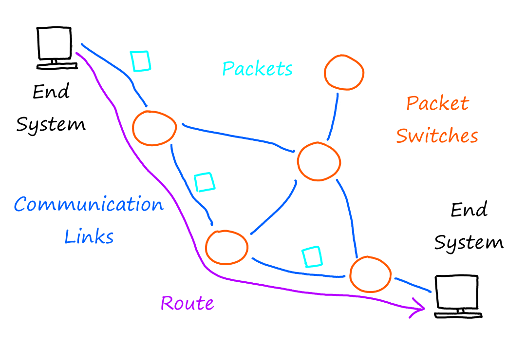
I believe the shape I'll be using for all packet switches is a circle/oval. And links will be just a line connecting the circles.
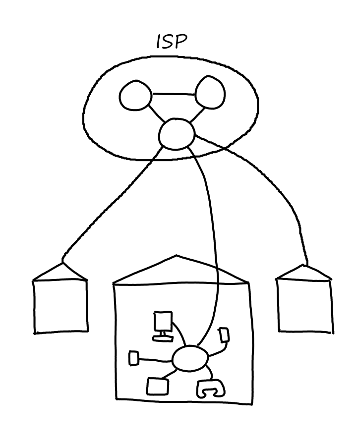
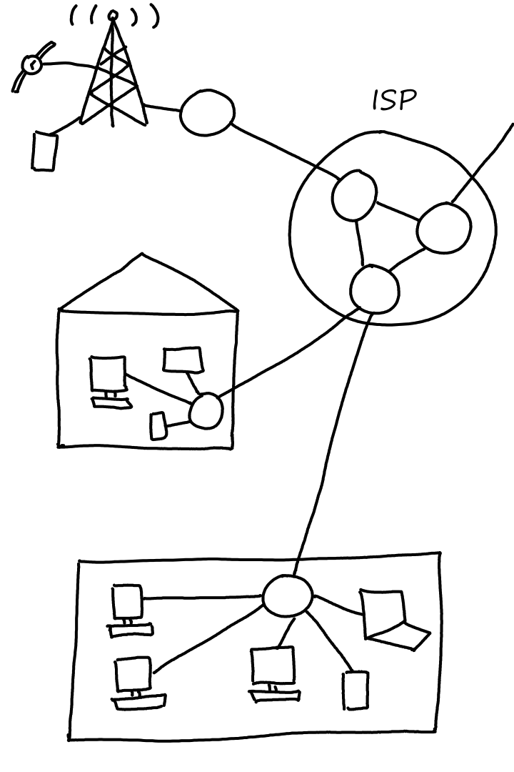
Access to the Internet is provided by Internet Service Providers (ISPs). Think ATT and Spectrum for example. ISPs themselves are a network of packet switches and communication links.
What is a Protocol?
All the devices involved with sending and receiving packets run protocols, which are a set of rules defining:
- how messages should be formatted
- the order of the messages exchanged
- the actions that can be performed when the messages are received or transmitted
The protocols are defined by Internet standards, which are developed by the Internet Engineering Task Force (IETF). The actual documents are called requests for comments (RFCs).
When we go to a URL on our browser, the actions that occur are a result of following a protocol (the TCP protocol).
- Computer sends a request to connect to the Web server and waits for a reply
- Web server receives the connection request and returns a "connection okay" message
- Computer sends the name of the Web page we want
- Web server sends it to our computer
Livin' on the Edge
The word "end system" is used to describe devices that connect to the Internet because they exist at the "edge" of the Internet.
Access Networks
The access network is the network where end systems connect to the first router in the path to the ISP. (There may be many routers in between the ISP and a home. The first router is the one that's actually in the home.) Basically, an access network is a network on the edge of the Internet.
Home Access: What's the WiFi Password?
The home network will probably be the easiest for everyone to relate to. All our phones, laptops, tablets, computers, and everything else that connect to the WiFi in our homes form a home network.
Two of the most popular ways to get Internet access are by a digital subscriber line (DSL) (think telephone lines and telephone companies) and cable.
Wide-Area Wireless Access: Unlimited Talk, Text, and Web For Only $ Per Month!
When our phones aren't connected to WiFi, it uses mobile data, which is Internet provided by cellular network providers through base stations (cell towers?). This is where the terms 3G, 4G, 5G, and LTE come into play. (6G doesn't exist yet at the time of this writing.)
The Network Core
The network core is, well, the part of the Internet that is not at the edge. This is the part of the Internet that our router connects to — out to where our Internet access comes from.
Packet Switching
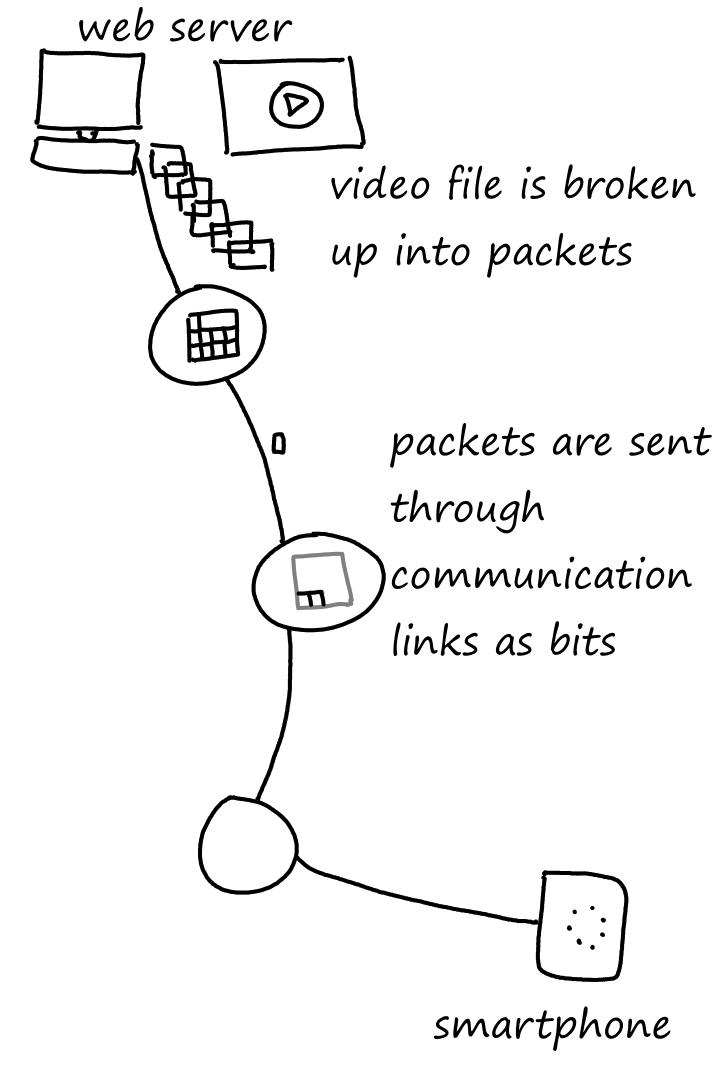
The data that the end systems send and receive are called messages. Messages can be any type of data, such as emails, pictures, or audio files. When going from their source to their destination, messages are broken up into packets, which are transferred from packet switch to packet switch. From packet switch to packet switch, each packet is broken up into bits and sent across the communication link connecting the two packet switches.
No Packet Left Behind
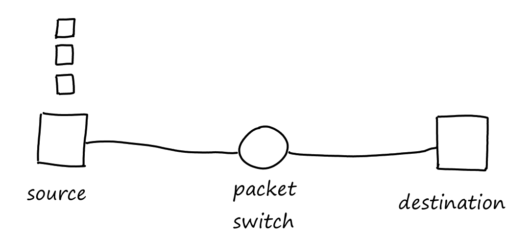
Most packet switches use store-and-forward transmission. This means that the packet switch waits until it receives the entire packet before it starts sending the first bit of the packet to the next location.
Consider a simple network of two end systems and one packet switch. The source has three packets to send to the destination.
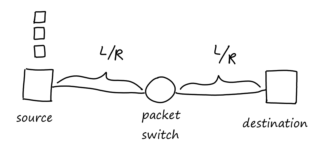
Let's say each packet has `L` bits and that each communication link can transfer `R` bits per second. Then the total time it takes to transfer one packet across one communication link is `L/R` seconds.
So the time it takes to transfer the packet from source to destination is `2L/R`.
How long does it take to transfer all three packets from source to destination? At `L/R` seconds, the packet switch receives all of the first packet. At this time, while the packet switch starts sending bits of the first packet to the destination, it also starts receiving bits of the second packet from the source.
At `2L/R` seconds, the first packet arrives at the destination and the second packet arrives at the packet switch.
At `3L/R` seconds, the second packet arrives at the destination and the third packet arrives at the packet switch.
At `4L/R` seconds, the third packet arrives at the destination.
Let's generalize this for `N` communication links and `P` packets.
It's helpful to think about this from the point of view of the last packet.
First, the last packet has to wait for the `P-1` packets ahead of it to be transmitted; this takes `(P-1)L/R` time.
Then it will be transmitted onto the link, which takes `L/R` time. Since there are `N` links, the total time the last packet will travel is `NL/R`.
So the total time it takes `P` packets to travel across `N` communication links is `(P-1)L/R+NL/R=(N+P-1)L/R`.
Besides store-and-forward, there's also cut-through switching, in which the switch starts sending bits before the whole packet is received.
Queuing Delays
Realistically, a packet switch has more than two links. For each link in the packet switch, there is an output buffer (a.k.a. output queue) where the packets wait if the link is busy. This can happen if the transmission rate of the link is slower than the arrival rate of the packets, i.e., the packets are coming in faster than the packet switch can send them out.

Okay, Some Packets Left Behind
Since the buffer can only be so big, if there isn't enough room for more incoming packets, some packets will be dropped, resulting in packet loss. Depending on the implementation, either the arriving packet or one of the packets in the buffer is dropped.
Forwarding Tables
Again, packet switches usually have multiple links. So how does the packet switch know which link to send the packet to? The answer is that each packet switch has a forwarding table that lists the destination of each link. When a packet arrives, the packet switch examines the packet to see its destination and searches it up in the packet's forwarding table. The table tells the packet switch which link to use to get to the destination.
Circuit Switching
With packet switching, the packets are sent and if there is a lot of traffic, then oh well. Maybe the data will take a long time to send — or worse — get dropped. To avoid this, we can reserve the resources ahead of time. This way, one connection won't be competing with other connections, i.e., the connection will have the links to itself. (Imagine being the only one on the road and no other cars are allowed to be on the road with you!)
With circuit switching, each link has a number of circuits. One circuit per link is required for communication between two end systems. So a link with, for example, four circuits can support four different connections at the same time. However, each connection only gets a fraction of the link's transmission rate.
Suppose we have a link with four circuits and a transmission rate of `1` Mbps. Then each circuit can only transfer data at a rate of `1/4` Mbps, which is `250` kbps.

Frequency-Division Multiplexing
Multiplexing is sending multiple signals as one big signal.
Multiple end systems can all use one link to transfer data if there are enough circuits. Each end system will be transferring different data, but they all get transferred over as "one big data" through the link. The way to differentiate which data came from which end system is to divide the link into different frequencies, such as in the example above.
Radio uses FDM. We can tune in to a specific frequency to listen to the station we want.
Time-Division Multiplexing
With time-division multiplexing, the end systems get to use all of the frequency to transfer data, but only for a limited amount of time.
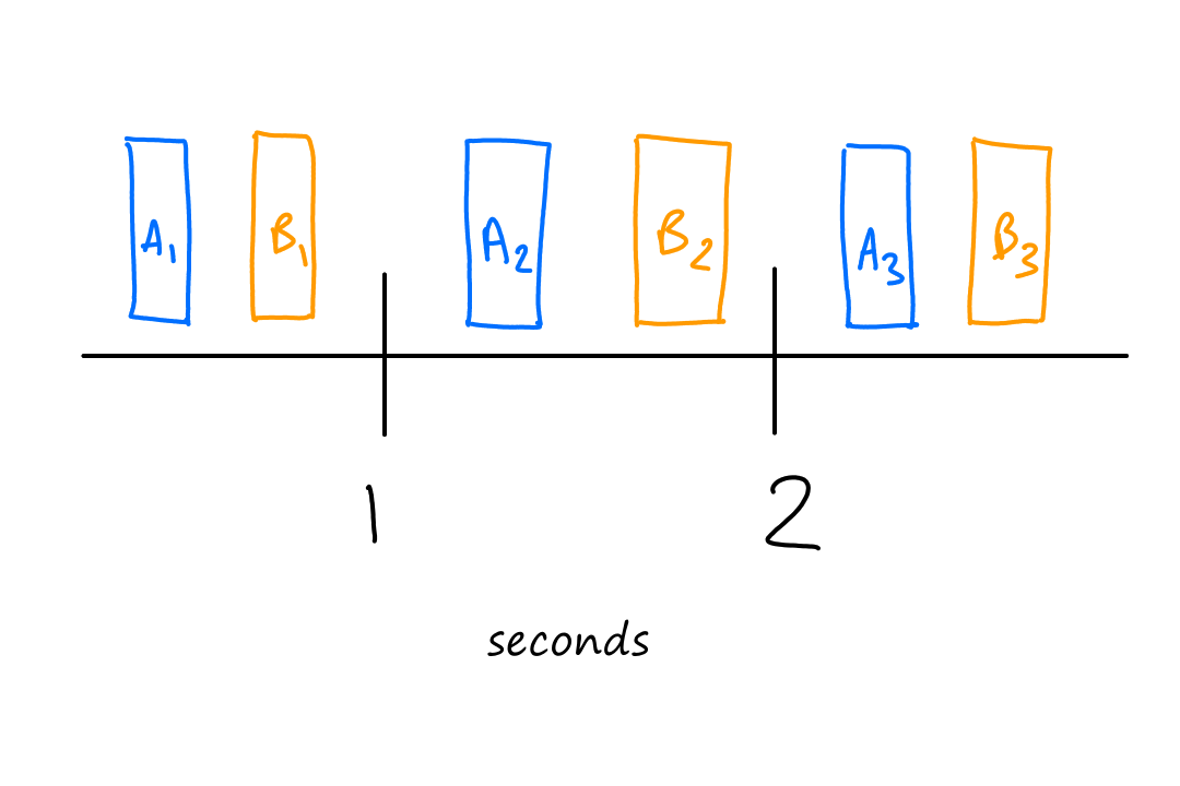
Suppose there are two end systems (`A` and `B`) communicating with two other end systems using the same link. Let's say they're only allowed `1`-second intervals to send their data. So from `0` to `1` seconds, part of the data from `A` and part of the data from `B` gets sent. From `1` to `2` seconds, part of the data from `A` and part of the data from `B` gets sent. And this repeats for every second.
More formally, time is divided into frames, and each frame is divided into slots. Once a connection between two end systems is established, one slot in every frame is reserved just for that connection.

If a link transmits `8000` frames per second and each slot consists of `8` bits, then the transmission rate of each circuit is `8000*8=64,000` bits per second `=64` kbps. The transmission rate of the whole link is `8000*8*text(number of slots)` (I think).
Suppose that all links in a network use TDM with `24` slots and can transfer data at a rate of `1.536` Mbps. Then each circuit has a transmission rate of `1.536/24=64` kbps.
Suppose there is a circuit-switched network with four circuit switches `A`, `B`, `C`, and `D`.
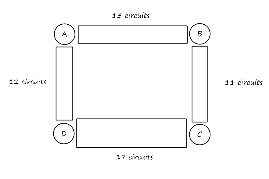
What is the maximum number of connections that can be ongoing in the network at any time?
There can be `13` connections from `A` to `B`, `11` connections from `B` to `C`, `17` connections from `C` to `D`, and `12` connections from `D` to `A`. So the maximum number of connections possible is `13+11+17+12=53`.
Note that while it's possible to have a connection from `A` to `C`, for example, that wouldn't maximize the number of connections because two circuits would have to be reserved for one connection, as opposed to the answer above where only one circuit has to be reserved for one connection.
Suppose that every connection requires two consecutive hops, and calls are connected clockwise. For example, a connection can go from `A` to `C`, from `B` to `D`, from `C` to `A`, and from `D` to `B`. What is the maximum number of connections that can be ongoing in the network at any time?
`ArarrBrarrC`: Since there are only `11` circuits from `B` to `C`, the number of connections possible for `ArarrBrarrC` is `11`.
`BrarrCrarrD`: Since all `11` circuits are being used for `ArarrBrarrC`, there are no circuits available for `BrarrCrarrD`.
`CrarrDrarrA`: Since there are only `12` circuits from `D` to `A`, the number of connections possible for `CrarrDrarrA` is `12`.
`DrarrArarrB`: Since all `12` circuits are being used for `CrarrDrarrA`, there are no circuits available for `DrarrArarrB`.
So the maximum number of connections possible is `11+12=23`.
Suppose that `13` connections are needed from `A` to `C`, and `19` connections are needed from `B` to `D`. Can we route these calls through the four links to accommodate all `32` connections?
For `ArarrC`, we can use the circuits for `ArarrBrarrC` and `ArarrDrarrC`. `ArarrBrarrC` only supports `11` connections, so the remaining `2` connections will need to use `2` of the circuits in `ArarrD`.
For `BrarrD`, we can't use the circuits for `BrarrC` because they are already being used for `ArarrBrarrC`. So the only circuits available are for `BrarrArarrD`. There are only `10` circuits available for `ArarrD` since `2` of them are being used for `ArarrDrarrC`. So there are only `10` circuits available for `BrarrArarrD`, which is not enough for the `19` connections that are needed for `BrarrD`.
So the answer is no.
It doesn't matter how we choose to divide up the connections. Notice that `13` connections are needed from `A` to `C`, but any path from `A` to `C`, whether it's `ArarrDrarrC` or `ArarrBrarrC`, will have all the circuits used up on that path. So the connections from `B` to `D` can only travel in the other direction, and neither direction can support `19` connections on its own.
(Also, the answer can be obtained by looking at the answer to the second question, but that's boring.)
Switching Teams
Packet switching is not good for things that require a continuous connection, like video calls. However, packet switching is, in general, more efficient than circuit switching.
Suppose several users share a `1` Mbps link. But each user is not using the connection all of the time, i.e., there are periods of activity and inactivity. Let's say that a user is actively using the connection 10% of the time, and generates data at `100` kbps when they are active. With circuit switching, this means the link can support `(1 text( Mbps))/(100 text( kbps))=10` users at once. The circuit must be reserved for all `10` users as long as they are connected, even if they're not using it all the time.
With packet switching, resources are not reserved, so any number of users can use the link. If there are `35` users, the probability that `ge 11` users are actively using the connection at the same time is ~`0.0004`, which means there is a ~`0.9996` chance that there are `le 10` simultaneous users at any time. As long as there are not more than `10` users at a time, there will be no queuing delay (if there are more than `10` users, there will be more data than the `1` Mbps link can handle). So packet switching performs just as well as circuit switching while allowing for more users at the same time.
Sticking with the same `1` Mbps link, suppose there are `10` users. One of the users suddenly generates `1,000,000` bits of data, but the other users are inactive. Suppose the link has `10` slots per frame. If all `10` slots are utilized, then the link can send `1,000,000` bits per second (`= 1` Mbps). However, under the rules of circuit switching, only one of the slots per frame will be used for that user. As a result, the link will only transfer `(1,000,000)/10=100,000` bits per second for that user's connection. So it will take `(1,000,000)/(100,000)=10` seconds to transfer all the data.
With packet switching, since no other users are active, the one user gets to send all `1,000,000` bits of data in `1` second since there will be no queuing delays.
Suppose users share a `2` Mbps link. Also suppose each user transmits continuously at `1` Mbps when transmitting, but each user transmits only `20%` of the time.
When circuit switching is used, how many users can be supported?
Only `2` users can be supported since each user transmits at `1` Mbps.
Suppose packet switching is used from now on.
Why will there be no queuing delay before the link if `le 2` users transmit at the same time?
If only `1` user is transmitting, then there will be traffic at a rate of `1` Mbps, which the link can handle. If `2` users are transmitting, then there will be traffic at a rate of `2` Mbps, which the link can also handle.
Why will there be a queuing delay if `3` users transmit at the same time?
If `3` users are transmitting, then there will be traffic at a rate of `3` Mbps. But since the link's transmission rate is only `2` Mbps, packets will be coming in faster than they can be transmitted.
What is the probability that a given user is transmitting?
`20%`
Suppose there are `3` users. What is the probability that at any given time, all `3` users are transmitting at the same time?
The probability of `1` user transmitting is `20%=0.2`. So the probability of `3` users transmitting is `0.2*0.2*0.2=0.008`.
A Network of Networks
We get our Internet access from an ISP. Of course, all of us don't get Internet access from the same ISP. There are different ISPs out there providing Internet access to different networks. But then how do our end systems communicate with other end systems? How do we communicate with servers and visit websites from different parts of the world for example? The answer is that the ISPs themselves are connected with each other. But what exactly does that look like?
One idea is that we connect every ISP with each other directly.
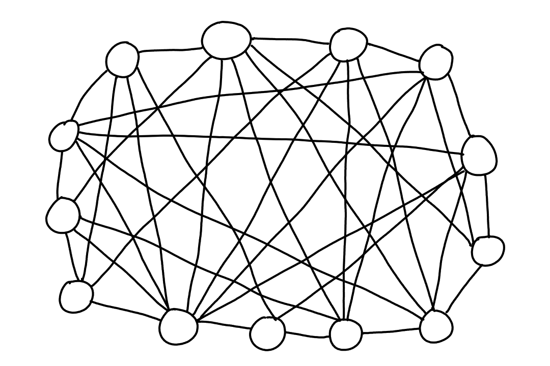
The problem with this is that it is too costly, because there would be way too many links (too many for me to draw). In computer science terms, there would be `n^2` connections.
To minimize the number of connections, another idea is that there is a global ISP and all the other ISPs connect to that global one.

While this is also costly, the global ISP would offset the cost by charging the other ISPs (we'll call them access ISPs from this point on) money to connect to the global ISP.
And if one global ISP becomes profitable, naturally there will be other global ISPs wishing to be profitable too.
This structure is good for the access ISPs because they can choose which global ISP they want to connect to by comparing prices and service quality. So what we have so far is a two-tier hierarchy where global ISPs are at the top and access ISPs are at the bottom.
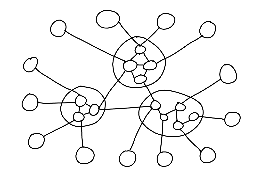
The reality is that these global ISPs can't exist in every city in the world. What happens instead is that the access ISPs connect to a regional ISP, which then connects to a global ISP. (We'll now be calling global ISPs by the more correct term tier-1 ISP.) Some examples of tier-1 ISPs are AT&T, Verizon, and T-Mobile.
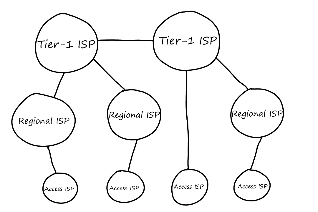
Sometimes, an access ISP can connect directly to a tier-1 ISP. In that case, the access ISP would pay the tier-1 ISP.
In some regions, there can be a larger regional ISP consisting of smaller regional ISPs.
Access ISPs and regional ISPs can choose to multi-home. That is, they can connect to more than one provider ISP at the same time, getting Internet access from multiple ISPs. While they have to pay each ISP they're connected to, the multi-homed ISPs can achieve better reliability in case one of the provider ISPs has a failure.
This multi-tier hierarchy is closer to the structure of today's Internet, but there are still a few pieces missing.
Lower-tier ISPs pay higher-tier ISPs based on how much traffic goes through their connection. To avoid sending traffic to the higher-tier ISPs, the lower-tier ISPs can peer. This means that they connect with each other so that the traffic goes between them instead of up to the higher-tier ISP.
For example, suppose that a computer connected to the green ISP wants to communicate with a computer connected to the blue ISP. Without peering, the traffic would have to go all the way up to the tier-1 ISP and back down from there.
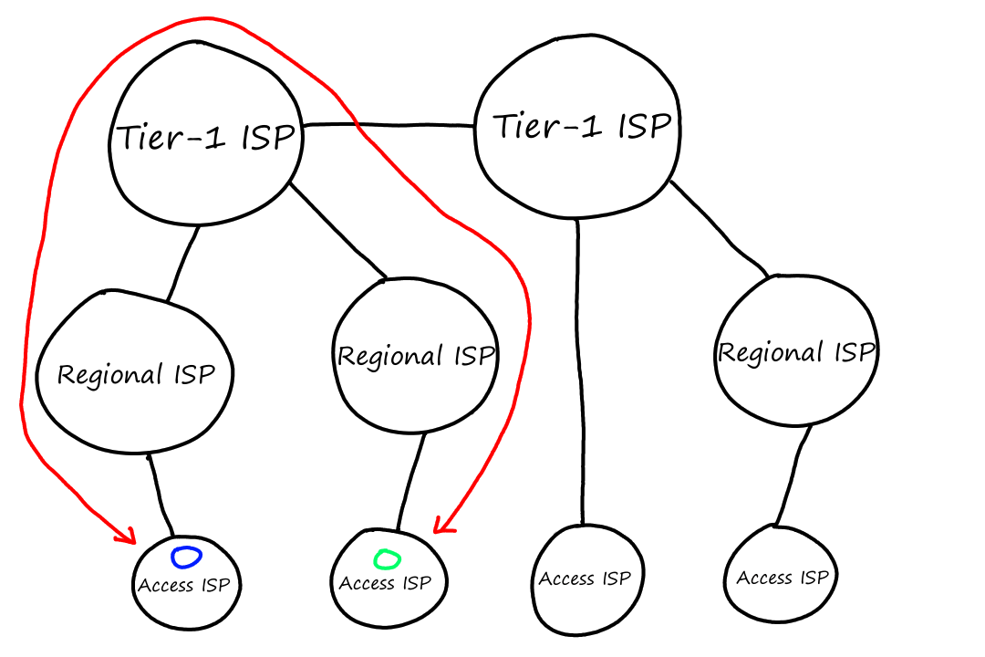
But with peering, they can avoid the cost of going through the regional and tier-1 ISPs by connecting with each other directly. Usually when ISPs peer with each other, they agree to not pay each other for the traffic that comes from peering.
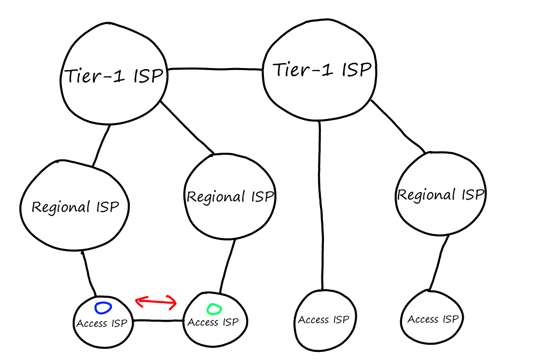
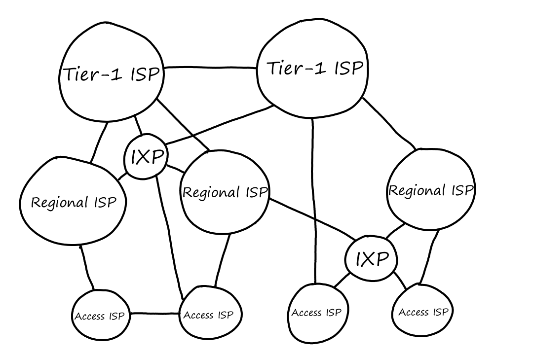
To facilitate this peering, third-party companies can create an Internet Exchange Point (IXP) which ISPs connect to in order to peer with other ISPs.
There's one more piece: content-provider networks. Content providers are companies such as Google, Amazon, and Microsoft.
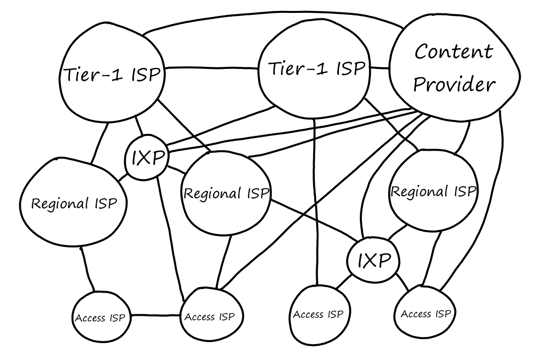
They run their own private networks so that they can bring their services and content closer to users. They do this by having data centers distributed everywhere across the world. Each data center has tons of servers that are all connected to each other.
And this is why the Internet is a network of networks. (Recall that ISPs themselves are networks of packet switches and links. There's also the edge network from the previous section, and each network in the edge network is a network of routers and links.)
Delay, Loss, and Throughput
In a perfect world, data would travel through the Internet instantaneously without any limitations. But, we know things aren't perfect.
What's the Holdup?
As packets travel along their route, they experience nodal processing delay, queuing delay, transmission delay, and propagation delay. All these delays combined is called total nodal delay.
Processing Delay
When a packet arrives at a router, the router looks at the packet's header to see which link it should go on. It also checks for any bit-level errors in the packet. The time it takes to do this (microseconds), is the processing delay.
Queuing Delay
Once the outbound link has been determined, the packet goes to the queue for that link. The time it waits in the queue (microseconds to milliseconds), is the queuing delay.
Transmission Delay
Once the packet reaches the front of the queue, it is ready to be transferred across the link. Recall that packets travel through links as bits. The time it takes to push all of the bits into the link (microseconds to milliseconds) is the transmission delay. If a packet has `L` bits and the link can transfer `R` bits per second, then the transmission delay is `L/R`.
Propagation Delay
Now that the bits are on the link, they must get to the other end. The time it takes to get from the beginning of the link to the end of the link (milliseconds) is the propagation delay. This is determined by two things: how fast the bits are able to move and how far they have to go. How fast the bits can move depends on the physical characteristics of the link (e.g., whether it's fiber optics or twisted-pair copper wire) and is somewhere near the speed of light.
If `d` is the distance the bit has to travel, i.e., the length of the link, and `s` is the propagation speed of the link, then `d/s` is the propagation delay.
Transmission delay and propagation delay sound very similar to each other. So here are some pictures illustrating the difference.
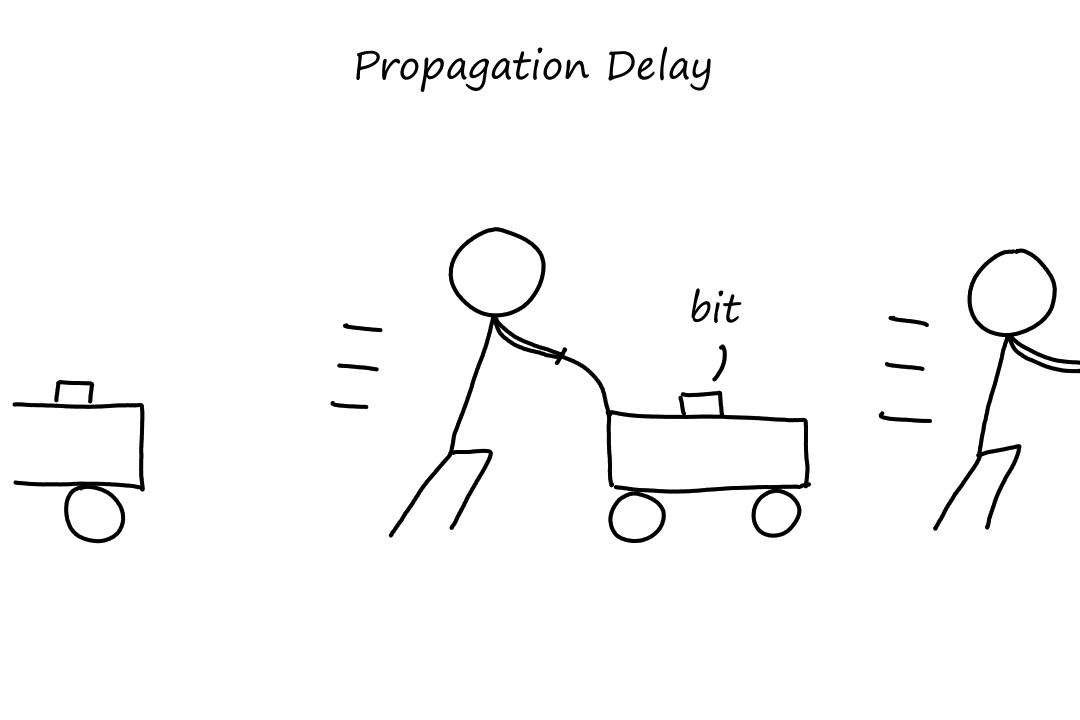
Yeah, somehow the bits go from being on a conveyer belt to being pushed in needlessly large carts. There's no delay from belt to cart though. That part happens magically.
Consider a packet of length `L` which begins at end system `A` and travels over three links to a destination end system. These three links are connected by two packet switches. For `i=1,2,3`, let `d_i`, be the length of each link, `s_i` be the propagation speed of each link, and `R_i` be the transmission rate of each link. The packet switch delays each packet by `d_text(proc)`. Assume there are no queuing delays.
In terms of `d_i`, `s_i`, `R_i`, and `L`, what is the total end-to-end delay for the packet?
The total end-to-end delay is the sum of all the delays: processing delay, queuing delay, transmission delay, and propagation delay.
The processing delay is given to us as `d_text(proc)`. There are two packet switches, so there will be two processing delays.
We are also given that there are no queuing delays.
The transmission delay is `L/R_1+L/R_2+L/R_3`.
The propagation delay is `d_1/s_1+d_2/s_2+d_3/s_3`.
So the total end-to-end delay is `d_text(proc)+d_text(proc)+L/R_1+L/R_2+L/R_3+d_1/s_1+d_2/s_2+d_3/s_3`.
Suppose now the packet is `1500` bytes, the propagation speed on all three links is `2.5*10^8` m/s, the transmission rates of all three links are `2` Mbps, the packet switch processing delay is `3` ms, the length of the first link is `5000` km, the length of the second link is `4000` km, and the length of the third link is `1000` km. What is the end-to-end delay?
From the first question, we know that the end-to-end delay is `d_text(proc)+d_text(proc)+L/R_1+L/R_2+L/R_3+d_1/s_1+d_2/s_2+d_3/s_3`, so now we'll just calculate and plug in those values.
We're given that `d_text(proc)=3` ms.
To calculate transmission delay, we'll first convert everything to bits. There are `8` bits in a byte, so the packet length is `1500*8=12,000` bits. For the transmission rate, `2` Mbps = `2,000,000` bits per second. Since all three links have the same transmission rate, `R_1=R_2=R_3`. So `L/R_1=L/R_2=L/R_3=(12,000)/(2,000,000)=0.006` seconds `=6` ms.
For the propagation delay, we'll first convert everything to meters. The lengths of the links are `5,000,000` m, `4,000,000` m, and `1,000,000` m. Since all three links have the same propagation speed, `s_1=s_2=s_3`. So `d_1/s_1=(5,000,000)/(250,000,000)=0.02` seconds `=20` ms, `d_2/s_2=(4,000,000)/(250,000,000)=0.016` seconds `=16` ms, and `d_3/s_3=(1,000,000)/(250,000,000)=0.004` seconds `=4` ms.
So the total-end-to-end delay is `3+3+6+6+6+20+16+4=64` ms.
Consider a highway that has a tollbooth every `100` km. It takes `12` seconds for a tollbooth to service a car. Suppose a caravan of `10` cars are on the highway with each car traveling `100` km/hour. When going from tollbooth to tollbooth, the first car waits at the tollbooth until the the other nine cars arrive. To analogize, the tollbooth is a router, the highway is a link, the cars are bits, and the caravan is a packet.
How long does it take the caravan to travel from one tollbooth to the next?
Since the tollbooth takes `12` seconds to service a car and there are `10` cars, it takes a total of `120` seconds (or `2` minutes) to service all the cars.
Since the distance between every tollbooth is `100` km and the cars are moving at `100` km/hour, it takes `1` hour (or `60` minutes) to reach the next tollbooth.
Since the cars in the caravan travel together, everything depends on the last car. So we'll look at this from the last car's point of view.
The last car has to wait `2` minutes before it can be serviced by the tollbooth. Once this is done, it takes `60` minutes for it to reach the next tollbooth. So it takes the last car `62` minutes to reach the next tollbooth.
Here's some animation to visualize:
At `120` seconds all `10` cars have exited the first tollbooth and are on the highway to the next tollbooth.
The first car will take `60` minutes to enter the next tollbooth (get off the animation line), but since it waited `12` seconds for the previous tollbooth servicing, it will enter the next tollbooth at `60:12`.
To analogize some more, the time it takes the tollbooth to service a car is the transmission delay. The time it takes the car to move to the next tollbooth is the propagation delay.
Now suppose that the cars travel at `1000` km/hour and the tollbooth takes `1` minute to service a car. Will cars arrive at the second tollbooth before all the cars are serviced at the first tollbooth? That is, will there still be cars at the first tollbooth when the first car arrives at the second tollbooth?
Now it takes `10` minutes to service all `10` cars.
The first car will wait `1` minute for the tollbooth to service it. Then it will take `6` minutes (`(100text(km))/((1000text(km))/(60text(min)))=6`) to reach the next tollbooth. So it will take a total of `7` minutes for the first car to go from one tollbooth to the next.
But in `7` minutes, the first tollbooth will have only serviced `7` cars. So there will be `3` cars still at the first tollbooth when the first car arrives at the second tollbooth.
Queuing Delay and Packet Loss
Queuing delay is the most complicated delay since it varies from packet to packet (as implied, processing delay, transmission delay, and propagation delay are the same for every packet). For example, if `10` packets arrive at an empty queue, the first packet will have no queuing delay, but the last packet will have to wait for the first `9` packets to leave the queue.
The factors that determine queuing delay are the rate at which traffic arrives, the transmission rate of the link, and the type of traffic that arrives (e.g., periodically or in bursts).
Let `a` be the average rate (in packets per second) at which packets arrive. If a packet has `L` bits, then `La` is the average rate (in bits per second) at which bits arrive. `R` is the transmission rate of the link. So `(La)/R` is the ratio of bits coming in vs bits going out; this ratio is called traffic intensity.
`(La)/R gt 1` means that bits are arriving at the queue faster than they are leaving. In this case, the queuing delay will approach infinity.
If `(La)/R le 1`, then the type of traffic that arrives has an effect on the queuing delay. For example, if one packet arrives every `L/R` seconds, then the packet will always arrive at an empty queue, so there will be no queuing delay.
However, if `N` packets arrive in bursts every `NL/R` seconds, then the first packet will experience no queuing delay. But the second packet will experience a queuing delay of `L/R` seconds. The third packet will experience a queuing delay of `2L/R` seconds. Generally, each packet will have a queuing delay of `(n-1)L/R` seconds.
Regardless of the type of traffic, as traffic intensity gets closer to `1`, the queuing delay gets closer to approaching infinity.
Average queuing delay grows exponentially with traffic intensity, i.e., a small increase in traffic intensity results in a large increase in average queuing delay.
Packet Loss
If packets are coming in faster than they are leaving the queue, then the queue will eventually be full and not be able to store any more packets. In this case, some packets will be dropped or lost. As traffic intensity increases, so does the size of the queue, which means the number of packets lost also increases.
End-to-End Delay
End-to-end delay is the total delay that a packet experiences from source to destination.
Suppose there are `N-1` routers between the source and destination. Then there are `N` links. Also suppose that the network is uncongested so there are practically no queuing delays.
Then the end-to-end delay is `d_text(end-end)=Nd_text(proc)+Nd_text(trans)+Nd_text(prop)=N(d_text(proc)+d_text(trans)+d_text(prop))`.
Traceroute
Traceroute is a program that allows us to see how packets move and how long they take. We specify the destination we want to send some packets to and the program will print out a list of all the routers the packets went through and how long it took to reach that router.
Suppose there are `N-1` routers between the source and destination. Traceroute will send `N` special packets into the network, one for each router and one for the destination. When the nth router receives the nth packet, it sends a message back to the source. When it receives a message, the source records the time it took to receive the message and where the message came from. Traceroute performs these steps 3 times.
Throughput
Throughput is the rate at which bits are transferred between the source and destination. The instantaneous throughput is the rate at any point during the transfer. The average throughput is the rate over a period of time.
If a file has `F` bits and the transfer takes `T` seconds, then the average throughput of the file transfer is `F/T` bits per second.
Suppose we have two end systems connected by two links and one router. Let `R_s`, `R_c` be the rates of the two links.
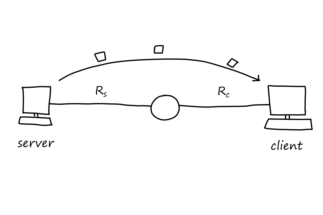
Suppose `F=32,000,000` bits, `R_s=2` Mbps, and `R_c=1` Mbps.
- After `1` second, `2,000,000` bits will move from the server to the router.
- After `2` seconds, `2,000,000` bits will move from the server to the router and `1,000,000` bits will move from the router to the client.
- After `3` seconds, `2,000,000` bits will move from the server to the router and `1,000,000` bits will move from the router to the client.
- After `4` seconds, `2,000,000` bits will move from the server to the router and `1,000,000` bits will move from the router to the client.
The file transfer is complete when the client receives `32,000,000` bits, which means `1,000,000` bits will have to move from the router to the client `32` times. Since it takes `1` second to do so, it will take `32` seconds for the file transfer to complete.
Notice how it didn't matter how fast the bits moved from the server to the router. The time the file took to reach the client only depended on the rate from the router to the client. This doesn't mean the time it takes to reach the client is always equal to the rate from router to client though. Let's flip the numbers around to prove this point.
Suppose `F=32,000,000` bits, `R_s=1` Mbps, and `R_c=2` Mbps.
- After `1` second, `1,000,000` bits will move from the server to the router.
- After `2` seconds, `1,000,000` bits will move from the server to the router and `1,000,000` bits will move from the router to the client.
- After `3` seconds, `1,000,000` bits will move from the server to the router and `1,000,000` bits will move from the router to the client.
- After `4` seconds, `1,000,000` bits will move from the server to the router and `1,000,000` bits will move from the router to the client.
Wait, but isn't the rate from router to client `2,000,000` bits per second? Why aren't `2,000,000` bits moving from router to client every second? That's because there are only `1,000,000` bits entering the router every second.
From this, we can see that the throughput of a file transfer depends on the link that is transferring bits at the lowest rate. This link is called the bottleneck link.
Mathematically, the throughput is `min(R_s,R_c)`.
The time it takes to transfer the file is `F/(min(R_s,R_c))`.
Generally, the throughput for a network with `N` links is `min(R_1,R_2,...,R_n)`.
The bottleneck link is not always the link with the lowest transmission rate. We'll look at another example to show this.
Suppose there are `10` clients downloading data from `10` servers (each client is connected to a unique server). Suppose they all share a common link with transmission rate `R` somewhere in the network core. We'll denote the transmission rates of the server links as `R_s` and the transmission rates of the client links as `R_c`.
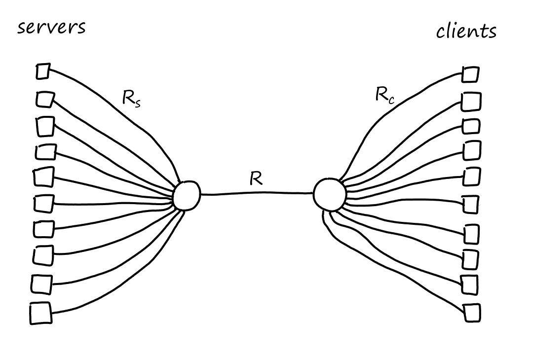
(I think sharing a common link means all the server links eventually connect to one router and all the client links eventually connect to a different router. And the link between these two routers are the same.)
Let's assign actual values to these transmission rates. So let `R_s=2` Mbps, `R_c=1` Mbps, and `R=5` Mbps. Since the common link is being used for `10` simultaneous downloads, the link divides its transmission rate equally among the `10` connections. So the common link is transferring bits at a rate of `(5text(Mbps))/10=500` kbps per connection. Which means the throughput for each download is `500` kbps. Even though the common link had the highest transmission rate, it ended up being the bottleneck link.
Links in the network core are almost never the bottleneck link because they are usually over-provisioned with high speed links. Typically, the bottleneck links are in the access network.
Protocol Layers
There are many pieces to the Internet, such as routers, links, applications ("apps"), protocols, and end systems. These pieces are organized into layers.
Layered Architecture: The Internet Is Like an Onion
The airline system can be seen as an organization of layers.
| Layer | Action (Leaving) | Action (Arriving) |
|---|---|---|
| Ticketing | Purchase | Complain |
| Baggage | Check | Claim |
| Gates | Enter | Exit |
| Runway | Takeoff | Land |
| Airplane | Routing | Routing |
Every time we board and leave an airplane, we perform the same steps in a certain order. And the action we perform depends on the layer we're at since each layer is responsible for one thing and one thing only. (I.e., each layer provides a different service.) Also, each layer depends on the layer before it. For example, we can only check in our baggage if we have a ticket, or we can only enter the gate once we have checked in our baggage.
This layering makes it easier to distinguish the different components of an airline system. It also makes it easier to change the implementation of a layer's service without affecting the rest of the layers. For example, the current implementation of the gate layer is to board people by ticket priority and check-in time. But the implementation can be changed to board people by height. This change doesn't affect any of the other layers, and the function of this layer remains the same: getting people on the airplane.
Protocol Layering
The Internet is made up of 5 layers.
| Layer |
|---|
| 5. Application |
| 4. Transport |
| 3. Network |
| 2. Link |
| 1. Physical |
Recall that a protocol is a set of rules that define how things should work. Each protocol belongs to one of the layers.
Application Layer
The application layer includes all the network applications (basically apps or programs that connect to the Internet).
| Protocol | Details |
|---|---|
| HTTP | sending and receiving Web documents |
| SMTP | sending emails |
| FTP | transferring files |
Applications communicate with each other by sending messages to each other.
Transport Layer
The transport layer is responsible for delivering the application's message to the network core.
| Protocol | Details |
|---|---|
| TCP |
connection oriented guaranteed delivery |
| UDP |
connectionless no reliability, no flow control, no congestion control |
In the transport layer, the packets of information are called segments.
Network Layer
The network layer is responsible for moving the transport layer's segments from router to router.
| Protocol | Details |
|---|---|
| IP |
defines how packets must be formatted defines the actions that must be taken when sending or receiving packets |
In the network layer, the packets are called datagrams.
Link Layer
The link layer is responsible for moving the network layer's datagrams across links.
| Protocol |
|---|
| Ethernet |
| WiFi |
| DOCSIS |
In the link layer, the packets are called frames.
Physical Layer
The physical layer is responsible for moving the individual bits of the link layer's frames across links.
OSI Model
In the late 1970s (before the Internet became public), there was another model that was proposed by the International Organization for Standardization (ISO) on how to organize computer networks. This model was called the Open Systems Interconnection (OSI) model and it had 7 layers:
| Layer |
|---|
| 7. Application |
| 6. Presentation |
| 5. Session |
| 4. Transport |
| 3. Network |
| 2. Link |
| 1. Physical |
The layers that also appear in the Internet model work roughly the same way. So we'll just go over the ones that are new.
The presentation layer makes sure the data is readable and usable. It provides data compression, data encryption, and data description. I guess it's sorta like a translator.
The session layer makes sure the data goes where it needs to go. It provides data synchronization, checkpointing, and data recovery.
Encapsulation
Whenever we moved across the different layers, we called the packets of information by a different name. That is because the packets change as they move from layer to layer.
- Application layer sends message
- Transport layer adds transport-layer header information to the message, forming a segment
- Network layer adds network-layer header information to the segment, forming a datagram
- Link layer adds link-layer header information to the datagram, forming a frame
The header information is needed so that the thing (e.g., router, link, end system) receiving the packet knows what it is and what to do with it. Here are some animations to illustrate:

End systems implement all 5 layers while routers usually implement only the bottom 3 layers (network, link, physical). (And some packet switches may only implement the bottom 2 layers, link and physical.)
Notice that when the packet left the end system, the last header added was the link-layer header, which is the first thing that gets processed when entering the router. When the packet reaches the link layer, the link-layer headers are extracted away. So now the top-most header is the network-layer header, which is what the network layer then processes.
After going through the network layer, the router determines that the packet has to go on another link again. So now the packet has to travel down the layers. When it goes from the network layer down to the link layer, a new link-layer header is added, so that the next thing (router or end system) can process it.
Now that the packet has reached the end system, it goes up the layers one last time. Again, at each layer the headers are removed until only the message remains, which the application understands.
From this point on, we'll go into more detail for each layer, starting with the application layer.
Principles of Network Applications
A network application is a set of apps or programs that connect to and communicate with the Internet. These apps are made by our local software developers using languages such as C, Java, or Python.
Typically, network applications involve multiple programs running on different end systems. For example, we can download Spotify on our phone, tablet, computer, or watch. And Spotify will have a different program running on their servers to provide functionality to the app.
Network Application Architectures
There are 2 types of network application architectures: client-server and peer-to-peer (P2P).
In the client-server architecture, there is a server that is always on and running. Whenever clients want data, they make a request to the server, which then provides the clients with what they requested. In addition to always being on, the server has a fixed IP address, so clients can make requests to the server at any time.
Big companies, like Google, need more than one server to handle all the requests, otherwise that one server would get overwhelmed. So they set up data centers, which house multiple servers. And then they go and set up multiple data centers.
In peer-to-peer architecture, there are no servers (and thus no clients). Instead, devices communicate directly with other devices — called peers — to transfer data.
Let's say you wanted to download a large file (perhaps an online textbook 🤫). You could go online and download it (this would be client-server), but let's say the file is so large, that it takes too long. Suppose that I happen to have the complete file already downloaded. Using the right application, I could transfer my file directly to your computer. Suppose that someone else also has the file. Then you can receive the file from both of us. And the more people that have the file, the more people you can connect to to receive the file, making the download faster.
The effectiveness of peer-to-peer relies on the number of peers. The more peers there are, the more computing power there is. This is referred to as self-scalability.
Processes Communicating
We call them programs. Operating systems call them processes.
Client and Server Processes
A network application consists of pairs of processes that send messages to each other. A Web broswer (a process) communicates with a Web server (another process). Spotify, the app (a process), communicates with Spotify's servers (another set of processes). The process that is requesting data is the client process and the process that is providing the data is the server process. Despite the naming, the terms "client" and "server" processes apply for both client-server architecture and peer-to-peer architecture.
More formally (and perhaps more accurately), client processes are the ones that initiate communication and server processes are the ones that wait to be contacted.
The Interface Between the Process and the Computer Network
As we saw before, a process in the application layer sends a message to the transport layer. In order to do so, it opens a socket, which is the application layer's door to the transport layer. Sockets are also used to receive messages from the transport layer.
For us developers, sockets are also referred to as the Application Programming Interface (API) between the application and the network. We don't have control over how the socket is implemented; that's handled by the OS.
Addressing Processes
In order for the message to go to the correct place, the sending process needs to specify where the message needs to be delivered to. First, it needs to specify which end system is receiving the message. This can be done by providing the IP address of the end system. Just knowing which end system is not enough though because an end system is running multiple applications while it's on, so we also need to know which application needs the message. Whenever processes open a socket, they must choose a number to "label" the socket. This number is called a port number. So by specifying the IP address and the port number, the message can be delivered to the correct application on the correct end system.
Transport Services Available to Applications
On the other side of the socket is a transport-layer protocol that delivers the message to the socket of the receiving process. There are several transport-layer protocols an application can choose from. When deciding which one to use, there are several things to consider.
Reliable Data Transfer
As we saw earlier, packets can get lost. For some situations, like transferring financial documents, packet loss is undesirable. But even though packets can get lost, a protocol can still guarantee that the file will be delivered correctly. If a protocol can provide this guarantee, then that protocol provides reliable data transfer.
In other situations, like video calls, some packet loss is acceptable. ("I'm sorry, can you repeat that? You cut out for a few seconds.") Those applications are referred to as loss-tolerant applications.
Throughput
Throughput is the rate at which bits are transferred between the source and destination (Hmm, I feel like I've said these exact words before 🤔). A transport-layer protocol can guarantee a specified throughput of some amount of bits per second. This would be useful for voice calls, which need a certain throughput in order for the voices to be heard clearly. Applications that have throughput requirements are bandwidth-sensitive applications.
Applications that don't are elastic applications. File transfers don't need a certain throughput. If more bits can be transferred, then the download will be faster. If fewer bits can be transferred, then the download will be slower.
Timing
Whereas throughput is the number of bits going through, timing is the delay between each bit. One timing guarantee might be that bits go to the receiving process every 100 milliseconds. For real-time applications, such as video calls and online games, it is ideal to have low delay.
Security
Before transferring the data, a transport protocol can encrypt it.
Transport Services Provided by the Internet
There are 2 transport protocols an application can use: TCP and UDP.
TCP
TCP is a connection-oriented protocol. The client and server have to confirm a connection (TCP connection) with each other first before messages can be transferred. And once the application is done sending messages, it must close the connection.
TCP also provides reliable data transfer. This means data is sent without error and in the proper order — there are no missing or duplicate bytes. Part of this is achieved by implementing congestion control. If the network is congested, the sending process will be throttled.
UDP
UDP is like the opposite of TCP. It's connectionless. The data transfer is unreliable — there's no guarantee all the messages will arrive and if it does arrive, there's no guarantee that the messages will arrive in order. And there's no congestion control. All of these things sound bad, so why does UDP even exist in the first place?
Well, no congestion control means that UDP can send bits at any rate with no limits*. This is good for voice call applications because they want data to be sent as much as possible and as fast as possible.
*However, there will be actual limitations to this rate, including link transmission rate and network congestion.
For some reason, most firewalls are configured to block most types of UDP traffic. So applications that use UDP have to be prepared to use TCP as a backup.
| Application | Application-Layer Protocol | Transport-Layer Protocol |
|---|---|---|
| SMTP | TCP | |
| Remote terminal access | SSH | TCP |
| Web | HTTP | TCP |
| File transfer | FTP | TCP |
| Streaming | HTTP | TCP |
| Internet telephony | SIP, RTP, etc. | TCP or UDP |
TCP and UDP both don't guarantee:
- throughput
- timing
- security*
Despite this, time-sensitive applications still work. This is because they are designed with these lack of guarantees in mind.
*TCP can be enchanced with Transport Layer Security (TLS) to provide encryption. TLS is not a protocol; it's an add-on to TCP.
Application-Layer Protocols
Application-layer protocols define:
- the types of messages exchanged (e.g., request and response messages)
- the format of the messages
- what fields can go in a message
- the meaning of the information in the fields
- rules for determining when and how processes send and respond to messages
Some protocols are defined in RFCs and are therefore public. While other protocols, such as Skype's, are proprietary.
The Web and HTTP
The Internet became big in the 1990s with the arrival of the World Wide Web.
Some Dry Facts About HTTP
A Web page is a document with a bunch of objects, which can be images, videos, JavaScript files, CSS style sheets, etc. (More formally, an object is a file that is addressable by a single URL.) A Web page is usually an HTML file that includes references to these objects. Web browsers request and display Web objects while Web servers store Web objects.
HTTP stands for HyperText Transfer Protocol, and it is the Web's application-layer protocol. When browsers request a Web page, they send HTTP request messages to the server and the server responds with HTTP response messages that contain the objects.
HTTP uses TCP as its transport protocol. Port 80 is reserved for HTTP, so when browsers and servers initialize their sockets, they use port 80.
HTTP is a stateless protocol. This means that the server does not store any information about the exchanges the server has with clients. For example, the server will not know if a particular client has asked for a Web page before or if it's the client's first time asking for the Web page.
The original version of HTTP is called HTTP/1.0. Then there was HTTP/1.1 (1997), HTTP/2 (2015), and HTTP/3 (2022).
Non-Persistent and Persistent Connections
Each time a browser makes a request for a Web page, the browser actually has to make a request for the base HTML file and then for each object in the file. In non-persistent connections, the browser opens a TCP connection for one object, then closes the connection after the object is sent. So a TCP connection has to be opened for each object. In persistent connections, the browser opens one TCP connection and requests/receives all the objects using that one connection. After one object is sent, the connection remains open for some period of time, allowing other objects to be sent using the same connection if needed. HTTP/1.1 and later use persistent connections by default.
HTTP with Non-Persistent Connections
- Browser starts a TCP connection to the server on port 80
- Browser sends an HTTP request message to the server
- Server receives the request, gets the base file, puts it in an HTTP response message, and sends the message
- Server closes the TCP connection
- Browser receives the response.
And these steps repeat for each object in the Web page. So if a Web page has `10` objects, there will be `11` connections made (`1` for the Web page and `10` for each object). If this seems tedious, it's because it is. That's why browsers can be configured to open multiple parallel connections at the same time instead of waiting for one connection to be done before opening another.
Let's look at one request in action:
As we can see, it takes some time for the client to receive the file after making a request.
The round-trip time (RTT) is the time it takes for a packet to travel from client to server. It includes queuing delay, processing delay, and propagation delay.
Notice that the definition of RTT is the time it takes for a packet — not an object — to travel from client to server and then back to the client. That is why transmission delay is not included in the definition of RTT.
RTT is a measure of how long it takes for the server to start getting back to the client, not how long it takes to completely get back to the client.

So the total response time is `2` RTTs plus the transmission time of the file. `1` RTT is for establishing the TCP connection and `1` RTT is for receiving the file.
Besides the delay for sending each object, there is also the burden of resource management. For each TCP connection, buffers and variables must be allocated; this can take up a lot of resources on the server if there are a bunch of connections to manage.
HTTP with Persistent Connections
Instead of closing the TCP connection after sending the requested object, the server keeps the connection open for a certain period of time so that multiple objects can be sent through the connection.
For both non-persistent and persistent connections, they can also be non-parallel or parallel. In non-parallel connections, the client waits until it receives an object before requesting another one. So each object requires `1` RTT. In parallel connections, the client requests an object as soon as it needs it, even if a previous request for an object has not been completed yet. This means if there are `n` objects, it could request for all `n` objects at once by opening `n` parallel connections. So it could take as little as `1` RTT to get all the objects. (Note that the `1` RTT is just for the objects in the base file. The browser still needs `1` RTT to get the base file itself first.)
Persistent parallel is the default in HTTP/1.1 (and later) and the example below will show why.
Note that parallel connections does not mean multiple links between client and server. If there is only one link between client and server and multiple objects are requested in parallel, I believe what happens is that the link transmits the objects in an alternating fashion.
Suppose there is a `100`-kilobit page that contains `5` `100`-kilobit images, all of which are stored on a server. Suppose the round-trip time from the server to a client's browser is `200` milliseconds. For simplicity, we'll assume there is only one `100` Mbps link between the client and server; the time it takes to transmit a GET request onto the link is zero. Note that based on the assumptions, the link has a `100` millisecond one-way propagation delay as well as a transmission delay (for the page and images).
For non-persistent, non-parallel connections, how long is the response time? (The time from when the user requests the URL to the time when the page and its images are displayed?)
Let's start with the base file. It takes `1` RTT to establish the TCP connection and another `1` RTT to start getting the base file. So there are a total of `2` RTTs for the base file. We are given that one RTT is `200` milliseconds, so the RTT is `200*2=400` milliseconds.
The transmission delay for the base file is `L/R=(100text( kb))/(100text( Mbps))=(100,000text( bits))/(100,000,000text( bits/s))=0.001` seconds `=1` millisecond.
So the total time it takes to get the base file is `400+1=401` milliseconds.
Now for the objects. Since it is non-persistent, the TCP connection for the base file will be closed and new ones (`1` each) will be needed for the objects. Since it is non-parallel, the previous TCP connection has to close before a new one opens.
For one object, it takes `1` RTT to establish the TCP connection, and `1` RTT to start getting the object. So `2` RTTs for one object. For `5` objects, this is a total of `5*2=10` RTTs. In terms of milliseconds, this is `200*10=2000` milliseconds.
The transmission delay for one object is the same for the base file. Then for `5` objects, the transmission delay is `1*5=5` milliseconds.
So the total time it takes to get all of the objects is `2000+5=2005` milliseconds.
Bringing the total time for the whole Web page to `2005+401=2406` milliseconds `=2.406` seconds.
What about for non-persistent, parallel connections?
Again, we'll start with the base file. It takes `1` RTT to establish the TCP connection and another `1` RTT to start getting the base file. So `2` RTTs. Same as before, `2*200=400` milliseconds for the RTTs for the base file.
The transmission delay is also the same at `1` millisecond.
So the total time it takes to get the base file is `400+1=401` milliseconds.
For the objects, since the connections are parallel, all `5` TCP connections will be opened in parallel in `1` RTT and all `5` objects will start to be retrieved at the same time in `1` RTT. So `2` RTTs for all `5` objects. This means it takes `2*200=400` milliseconds for the RTTs of all `5` objects.
Even though the connections are parallel, the objects are not transmitted onto the link in parallel. As we saw before, it takes `1` millisecond to transmit `1` object. So for `5` objects, `5` milliseconds.
So the total time it takes to get all of the objects is `400+5=405` milliseconds.
Bringing the total time for the whole Web page to `401+405=806` milliseconds `=0.806` seconds.
What about for persistent, non-parallel connections?
We open the TCP connection and wait for the base file to transmit and propagate, which takes `401` milliseconds.
For the objects, since the connection is persistent, we don't need to open any more TCP connections.
But since it is non-parallel, we need to get the objects one at a time. `1` RTT for each object means `5` RTTs for all objects, which means `5*200=1000` milliseconds for the RTTs.
And `5` milliseconds to transmit.
So the total time it takes to get all of the objects is `1000+5=1005` milliseconds.
Bringing the total time for the whole Web page to `401+1005=1406` milliseconds `=1.406` seconds.
What about for persistent, parallel connections?
The base file takes `401` milliseconds to transmit and propagate.
We don't need to open any more TCP connections, and all `5` objects will start to be retrieved at once in `1` RTT. So `200` milliseconds.
`5` milliseconds to transmit.
So the total time it takes to get all of the objects is `200+5=205` milliseconds.
Bringing the total time for the whole Web page to `401+205=606` milliseconds `=0.606` seconds.
HTTP/2
If we use only one TCP connection, we run into a problem called Head of Line (HOL) blocking. Let's say the base file has a large video clip near the top and many small objects below the video. Being near the top, the video will be requested first. Especially if the bottleneck link is bad, the video will take some time to transfer, causing the objects to have to wait for the video. The video at the head of the line blocks the objects behind it. Using parallel connections is one way to solve this problem, but multiple connections means the server has to open and maintain multiple sockets, which is not good if it can be avoided.
Standardized in 2015, HTTP/2 introduced a way to allow for using one TCP connection without experiencing HOL blocking.
HTTP/2 Framing
The solution is to break each object into small frames and interleave them. That way, each response will contain parts of each object.
Let's say the base file has `1` large video clip and `8` small objects. Suppose the video clip is broken up into `1000` frames and each of the small objects is broken up into `2` frames. The first response can contain `9` frames: `1` frame from the video and the first frame of each of the small objects. The second response can also contain `9` frames: `1` frame from the video and the last frame of each of the small objects. In just `18` frames, all of the small objects will have been sent. If the frames weren't interleaved, the small objects would be sent after `1016` frames.
(For some reason, interloven sounds right.)
Server Pushing
Another feature HTTP/2 introduced was server pushing, where the server can analyze the base file, see what objects there are, and send them to the client without needing to wait for the client to ask for them.
HTTP Message Format
There are two types of HTTP messages: request messages and response messages.
Request Messages: Give Me What I Want!
Here's an example of what a request message might look like:
GET /projects/page.html HTTP/1.1
Host: www.myschool.edu
Connection: close
User-agent: Mozilla/5.0
Accept-language: fr
The first line is the request line. There are three fields: the method field, the URL field, and the HTTP version field. As we can infer, the method is GET, which is the method for requesting objects (because, you know, we want to "get" them).
The lines below the request line are the header lines. Connection: close means "close the connection after giving me what I requested", i.e., use a non-persistent connection. Connection: keep-alive would be for a persistent connection. The user agent specifies what type of browser is making the request. And Accept-language: fr means get the French version if it exists.
It may look like the header line specifying the host is unnecessary, because the browser needed to know the host in order to establish the TCP connection in the first place. It turns out that it is needed by Web proxy caches, which we'll see later.
There is also an entity body that follows the header lines. It wasn't included in the example above because the entity body is usually empty for GET requests. The entity body is usually used for POST requests, which are used to submit information, like user inputs from a form. The information that needs to be submitted are included in the entity body.
This is a little bit unconventional, but GET requests can also be used to submit information. Instead of going in the entity body, the inputted data is included in the URL with a question mark, like google.com/search?q=what+is+http, where q is the name of the input and the stuff after the '=' is the value of the input.
Response Messages: Here You Go, Now Leave Me Alone!
Here's an example of what a response message might look like:
HTTP/1.1 200 OK
Connection: close
Date: Sat, 16 Sep 2023 19:23:09 GMT
Server: Apache/2.2.3 (CentOS)
Last-Modified: Sat, 16 Sep 2023 18:34:09 GMT
Content-Length: 6821
Content-Type: text/html

(the requested data...)
The first line is the status line. There are three fields: the protocol version, the status code, and the status message.
The lines below are the header lines. The Date: header line specifies when the HTTP response was created and sent by the server. The Server: header line specifies the type of the Web server. Last-Modified: is when the object was created or last modified. Content-Length: specifies the object's size in bytes.
The entity body contains the actual object (the requested data).
Cookies! 🍪
HTTP is stateless, so the server doesn't store information about the requests that the clients are making. However, servers sometimes want a way to identify users so that they can restrict access or provide user-specific information when responding to the client. This is where cookies come in. Cookies allow sites to keep track of users*.
*Technically, cookies keep track of browsers. But users usually use one browser, and that browser is usually used by only one user (unless it's a shared computer). So tracking a browsing session is essentially tracking a user.
Let's say we go to our favorite shopping site on our favorite browser. The site will create a unique ID (let's say 9876) for this request, store the ID in its database, and send the ID back in the response. The response will include a Set-cookie: header; this tells the browser to create and store a cookie file. For example, the header will look like Set-cookie: 9876, so the browser will store 9876 in a file. Now, as we navigate through our shopping site, the site can ask the browser to include this cookie in every request. Then the site will query its database for this ID to identify the user. If the ID exists in the database, the site will know the user has visited before, and if the ID isn't in the database, the site will consider this a new user visiting for the first time.
When we say that the site can identify a user, the site doesn't actually know who we are, like our name and stuff. Until we enter that information ourselves. When we enter our information to buy something or to fill out a form, the site can store that information and associate that with the ID in the cookie. So the next time we visit that site, it can look at the ID and the information linked to that ID.
Web Caching
A Web cache is a server that stores Web pages and objects that have been recently requested.
When a browser requests an object, it sends the request to a Web cache. If the Web cache has a copy of the requested object, the Web cache sends it to the browser. If it doesn't, the Web cache requests it from the origin server, which sends the object to the Web cache. The Web cache stores a copy of it in its storage and sends that copy to the browser.
Having a Web cache can significantly speed things up. If the server is physically located far away from the client or if the bottleneck link between the server and client is really bad, then using a Web cache can reduce response times, assuming the Web cache is physically closer to the client or the bottleneck link between the Web cache and client is faster than the bottleneck link between the server and client.
Let's look at a hypothetical access network connected to the Internet. The router in the access network is connected to the router in the Internet by a `15` Mbps link. The links in the access network have a transmission rate of `100` Mbps. Suppose the average object size is `1` Mbits and that the average request rate is `15` requests per second. Also suppose that it takes `2` seconds on average for data to travel between the router in the Internet and the origin servers (we'll informally call this "Internet delay"). And that it takes `0.01` seconds on average for data to travel in the access network.
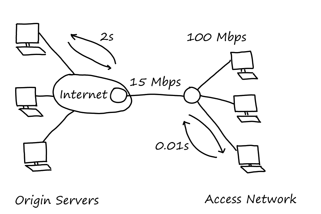
Recall that traffic intensity is `(La)/R` where `La` is the average rate at which bits are traveling and `R` is the transmission rate of the link.
On the access network, `15` requests per second and `1` Mbits per request means there are `15` Mbits traveling per second. So the traffic intensity is
`(La)/R=15/100=0.15`
which isn't too bad. In fact, the delay on the access network is negligible for a traffic intensity of `0.15`.
On the access link, the traffic intensity is
`(La)/R=15/15=1`
which is really bad. The average response time could be in minutes. (Recall that queuing delay increases as traffic intensity approaches `1`.)
One solution is to upgrade the access link, but that's costly.
Instead, let's consider placing a Web cache in the access network. Suppose that there is a `40%` chance that the cache can satisfy a request (i.e., the hit rate is `0.4`). This means only `60%` of the requests are going through the access link, so the traffic intensity is `1*0.6=0.6`.
The average delay is the sum of the access network delay, access link delay, and Internet delay. The access network delay is `0.01` seconds; the access link delay is negligible with a traffic intensity of `lt 0.8`; and the Internet delay is `2` seconds. Since `40%` of the requests stay in the access network and `60%` of the request go to the Internet, the average delay is
`0.4*(0.01+0+0)+0.6*(0.01+0+2)=0.004+1.206=1.21` seconds
If we had upgraded the access link instead of using a Web cache, the average delay would be at least `2` seconds from the Internet delay alone. So we can see that using a Web cache provides faster response times.
Conditional GET
The problem with using a Web cache is that objects in the Web cache can get outdated since the Web cache only stores a copy of the object while the actual object sits at the server and can be modified. The simple fix is for the Web cache to send a request to the server to check the last time the object was modified.
Let's say the browser sends a request to the Web cache. Suppose the Web cache doesn't have it, so it will send a request to the server. The server will send the object to the Web cache:
HTTP/1.1 200 OK
Date: Sun, 17 Sep 2023 19:10:09
Server: Apache/1.3.0 (Unix)
Last-Modified: Sun, 17 Sep 2023 18:30:09
Content-Type: image/gif

(the requested data...)
Now, the Web cache will send the object to the browser and make a copy of the object. Let's say the browser requests the same object one week later. The Web cache has a copy of the object this time, but it will send a conditional GET to the server first to check if there have been any changes:
GET /fruit/kiwi.gif HTTP/1.1
Host: www.exotiquecuisine.com
If-modified-since: Sun, 17 Sep 2023 18:30:09
Let's say the object hasn't been modified since then. The server will then send this to the Web cache:
HTTP/1.1 304 Not Modified
Date: Sun, 24 Sep 2023 15:39:09
Server: Apache/1.3.0 (Unix)
The entity body will be empty since it is pointless to send the object. However, if the object had been modified, the object would have been sent in the entity body.
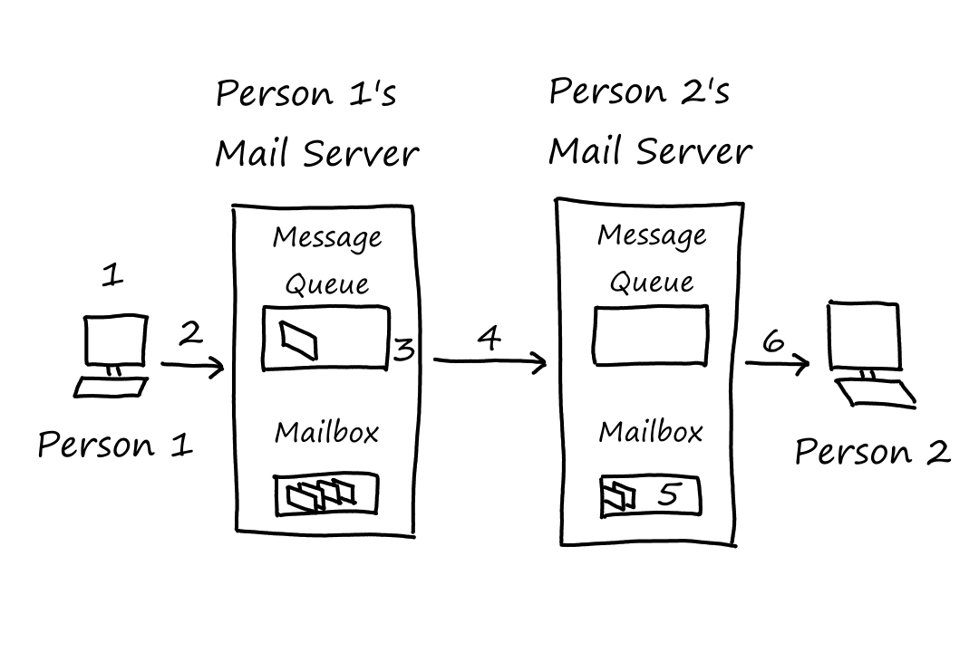
The Internet's mail system has three components: user agents, mail servers, and the Simple Mail Transfer Protocol (SMTP). User agents are applications, such as Gmail and Outlook, that allow us to read and write emails. Mail servers store emails in mailboxes and send emails to other peoples' mailboxes. Before being sent, emails wait in the sender's mail server's message queue.
We, as individuals, have our own mail servers (in a sense). This may sound a little weird (what? I'm running a server?). When we create an email account on, say, Google, Google manages a mail server for us. This mail server is shared with other Google users. (Note, the mail server is shared, not the mailbox.)
SMTP
SMTP is the application-layer protocol for email applications. Specifically, it is the protocol for sending emails (not receiving). It uses TCP as the underlying transport-layer protocol (which is probably not surprising). When a mail server sends mail, it is an SMTP client. When a mail server receives mail, it is an SMTP server.
SMTP requires emails to be encoded using 7-bit ASCII. This restriction is a result of SMTP being around since the 1980s, when people weren't sending a lot of emails, much less emails with large attachments like images and videos.
- Person 1 uses their user agent to write and send an email
- Person 1's user agent sends the email to Person 1's mail server, which places the email in its message queue
- Person 1's mail server opens a TCP connection to Person 2's mail server
- After TCP's whole handshaking thing, Person 1's mail server sends the email
- Person 2's mail server receives the email and puts it in Person 2's mailbox
- Person 2 uses their user agent to read the email
Person 1's user agent sends emails to Person 1's mail server, which then sends emails to Person 2's mail server. It may seem more efficient for Person 1's user agent to send emails directly to Person 2's mail server. This won't work though because user agents don't have a way to deal with Person 2's mail server being unreachable for whatever reason. Mail servers, which are always on and always connected to the Internet, keep retrying every `n` minutes until it works.
SMTP uses persistent connections. So if a mail server has multiple emails to send to the same mail server, then it can use the same TCP connection to send all the emails.
In HTTP, each object is sent in its own response message. In SMTP, all of the objects are placed into one email.
After the TCP handshake, there is another SMTP handshake that takes place between the mail servers before they can send and receive emails.
Mail Message Formats
An email consists of a header and a body. The header is kinda like the metadata of the email. An example:
From: me@gmail.com
To: you@gmail.com
Subject: Thanks for reading this
And, of course, the body contains the message.
Mail Access Protocols
As mentioned eariler, SMTP is used only for sending emails. For receiving emails, there are two main protocols. Web-based applications, like Google's Gmail website and app, use HTTP. Some other clients, like Outlook, use Internet Mail Access Protocol (IMAP).
Both of these protocols also allow us to manage our emails. For example, we can move emails into folders, delete emails, and mark emails as important.
Mail servers only use SMTP to send emails. User agents on the other hand, can use SMTP or HTTP to send emails to the mail server.
DNS
As we probably know, computers like to work with numbers. So naturally, servers are uniquely identified by a set of numbers (IP address). However, we don't type a bunch of numbers if we want to go to Google — we type "google.com" (does anyone actually type this to Google something?). "google.com" is what's known as a hostname, which is a human-readable name for a server.
Services Provided by DNS
The Internet's domain name system (DNS) is what allows us to type human-readable names to go to websites. It converts human-readable hostnames to IP addresses.
DNS is a distributed database deployed on a bunch of DNS servers.
It is also an application-layer protocol that allows hosts to query the database. It uses UDP.
Here's how it works:
- There is a DNS application running on our phone/computer
- The browser sends the hostname to the DNS application
- The DNS application uses the hostname to query a DNS server for the IP address
- The DNS application receives the IP address and sends it to the browser
- The browser uses the IP address to open a TCP connection
From this, we can see yet another source of delay: translating the hostname to an IP address.
DNS also provides additional related services. Sometimes, a hostname can be complicated, like "relay1.west-coast.enterprise.com". An alias can be set up so that we can type "enterprise.com" instead of that long hostname. The long (real) hostname is called the canonical hostname. This is called host aliasing. Something similar is available for mail servers too. "gmail.com" is more likely an alias than an actual hostname for a mail server (which could be something like "relay1.west-coast.gmail.com"). This is mail server aliasing.
Companies often have several servers running their website. Each server has its own IP address, but those IP addresses should all point to the same website. The DNS database stores this set of IP addresses and rotates between the IP addresses so that traffic is distributed evenly across all servers. So DNS also provides load distribution.
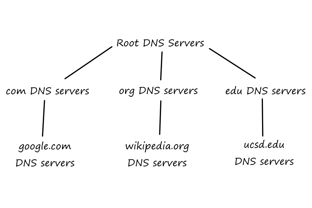
How DNS Works
DNS is a distributed database organized in a hierarchy. At the top are root DNS servers. This is where the translation starts. The DNS application queries the root DNS server, which then looks at the top-level domain (e.g., com, org, edu, gov, net). It does this because there are dedicated DNS servers for each top-level domain (i.e., there are DNS servers for all .com websites, DNS servers for all .edu websites, etc.). Appropriately, they're called top-level domain (TLD) servers. So the root server will tell the DNS application which TLD server to contact. The TLD server will send back to the DNS application the IP address of the authoritative DNS server, which is where the actual IP address of the website sits. So finally, the DNS application will contact the authoritative DNS server for the IP address of the website.
There's also a local DNS server, which aren't part of the hierarchy for some reason. The local DNS server is the entry point into the DNS hierarchy; the DNS application first contacts the local DNS server, which then contacts the root DNS server. Local DNS servers are managed by ISPs.
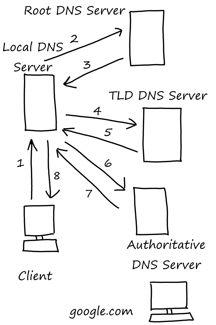
1. Local DNS! What is google.com's IP address?
2. Root DNS! What is google.com's IP address?
3. Go ask a com TLD server. Here's the IP address of one.
4. TLD DNS! What is google.com's IP address?
5. Go ask one of Google's authoritative servers. Here's the IP address of one.
6. Authoritative DNS! What is google.com's IP address?
7. The IP address is 127.0.0.1.
8. I finally know google.com's IP address. It's 127.0.0.1.
In the example above, the queries from the local DNS server (2, 4, and 6) are iterative queries. This means that the responsibility of asking the next query is placed on the server that asked the query.
There are also recursive queries, in which the responsibility of asking the next query is placed on the server who got asked. In the example above, 1 is a recursive query.
Here's an example where all the queries are recursive.
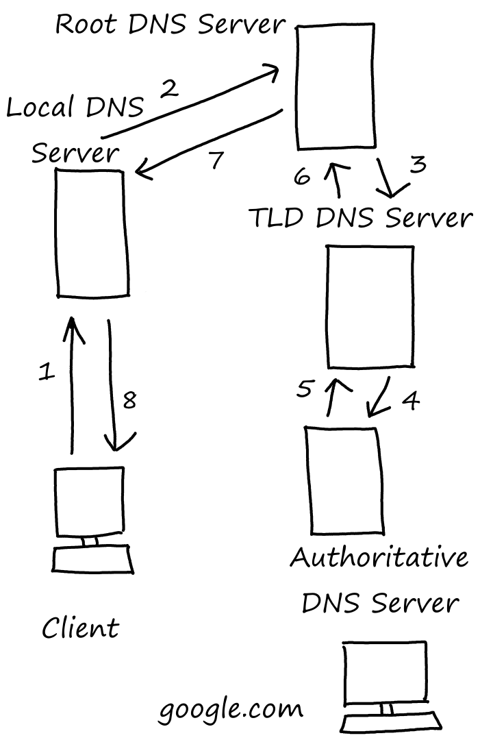
1. Local DNS! What is google.com's IP address?
2. Root DNS! What is google.com's IP address?
3. TLD DNS! What is google.com's IP address?
4. Authoritative DNS! What is google.com's IP address?
5. TLD DNS! The IP address is 127.0.0.1.
6. Root DNS! The IP address is 127.0.0.1.
7. Local DNS! The IP address is 127.0.0.1.
8. I finally know google.com's IP address. It's 127.0.0.1.
In practice though, most queries are iterative.
DNS Caching
As we saw earlier, there are a lot of queries that get made when going through the hierarchy. This traversal can be skipped if the DNS server stores the IP address of whatever was queried. For example, a local DNS server can store the IP address of a website, so that if another host wants to visit the same website, the local DNS server doesn't have to ask all those other DNS servers; it just returns the IP address it stored. This cache isn't good for very long though (typically 2 days).
Especially for .com websites, root DNS servers are often bypassed since the local DNS server should typically have the IP address of the appropriate TLD server in its cache. How many .com websites do we (as a whole) go to in a day?
DNS Records and Messages
The entries in the database are called resource records. A resource record is a four-tuple that looks like this: (Name, Value, Type, TTL). TTL stands for "time to live", which indicates when the record should be removed from a cache. The name and value depend on what the type is. (We'll ignore the TTL in the examples below.)
Type A records are hostname-to-IP mappings. (relay1.abc.def.com, 145.37.93.126, A). The name is the hostname and the value is the IP address for that hostname.
Type NS records are domain-to-DNS-server mappings. (abc.com, dns.abc.com, NS). The name is a domain and the value is the hostname of a DNS server.
CNAME records are alias-to-canonical-hostname mappings. (abc.com, relay1.abc.com, CNAME). The name is an alias and the value is the canonical hostname.
MX records are the equivalent of CNAME records but for mail servers. (abc.com, mail.abc.com, MX).
Type AAAA records are also hostname-to-IP mappings, but for IPv6.
Inserting Records into the DNS Database
If we want to register a domain name, say "ourwebsite.com", we do so through a registrar. A registrar makes sure the domain is unique and inserts the appropriate records into the DNS database.
The registrar also needs the names and IP addresses of the primary and secondary authoritative DNS servers. Once that is provided, the registrar inserts a Type NS record and a Type A record into the appropriate TLD server. For example, (ourwebsite.com, dns1.ourwebsite.com, NS) and (dns1.ourwebsite.com, 199.199.199.199, A) are inserted into the TLD servers for .com websites. So when a (local) DNS server contacts a TLD server, the TLD server will return both the Type NS record and the Type A record.
nslookup is a tool for performing DNS queries.
Here's a sample output for nslookup google.com:
Server: dns-cac-lb-01.rr.comAddress: 3002:1997:f01:1::1Non-authoritative answer:Name: google.comAddresses: 2607:f8b0:4007:80f::200e172.217.14.110
The Server is the DNS server to which the query is sent. If no DNS server is specified in the command, then it is the default DNS server, which is usually the local DNS server.
Non-authoritative answer means the answer is not from an authoritative DNS server. What happened was that the local DNS server queried a non-authoritative server that had the answer in its cache.
Here, there happened to be two answers returned. 2607:f8b0:4007:80f::200e and 172.217.14.110 are two separate servers for google.com.
Here's a sample output for nslookup -type=NS google.com:
Server: dns-cac-lb-01.rr.comAddress: 3002:1997:f01:1::1Non-authoritative answer:google.com nameserver = ns2.google.comgoogle.com nameserver = ns1.google.comns1.google.com internet address = 216.239.32.10ns2.google.com internet address = 216.239.34.10
This time, we're asking for Type NS records, so we'll see hostnames instead of IP addresses in the (first two lines of the) answer. Specifically, these are the hostnames for Google's authoritative DNS servers.
In the second half of the answer are Type A records for the authoritative DNS servers. Even though we didn't ask for Type A records, the local DNS server gave it to us for free.
Here's a sample output for nslookup google.com ns2.google.com:
Server: ns2.google.comAddress: 2001:4860:4802:34::aName: google.comAddresses: 2607:f8b0:4007:809::200e142.250.176.14
This command is sending the query to a specified DNS server (ns2.google.com) instead of to the local DNS server. Note that there's no Non-authoritative answer; this makes sense because we're querying an authoritative DNS server for google.com.
We might expect the address of the DNS server to match the address from the previous Type NS query, since they're both ns2.google.com. Depending on configurations, queries will return either an IPv4 or IPv6 address. So for all we (I) know, they may be the same server. Also, there are other reasons why IP addresses might not match in general: cache expiration, round robin (refer to DNS load distribution), and server scaling are a few.
ipconfig (on Windows) is a tool that allows us to see IP addresses of things.
Here's a sample partial output for ipconfig /all:
Wireless LAN adapter Wi-Fi:IPv6 Address. . . . . . . . . . . : 3912:6001:f122:5b21:b5c7:284d:6b93:3a12(Preferred)Temporary IPv6 Address. . . . . . : 3912:6001:f122:5b21:e6a2:778a:3c12:ab92(Preferred)IPv4 Address. . . . . . . . . . . : 173.146.1.189(Preferred)DNS Servers . . . . . . . . . . . : 3002:1997:f01:1::1
There will likely be many network interfaces shown, but since I'm connected to the Internet via WiFi, the WiFi one is the relevant one. Note that the IP address of the DNS server matches the IP address from nslookup.
Peer-to-Peer File Distribution
We saw this earlier, but in peer-to-peer applications, there are no servers sending data to clients. Instead, devices connect to each other and are called peers. Specifically for file distribution, peers send/receive portions of files to/from other peers.
It may be weird to think that only portions of files get distributed. While it's possible for a peer to have the whole file in storage, the peer may choose/have to only share a portion of the file with other peers for whatever reason. The peers who only got a portion of the file will share whatever they got with other peers who don't have it yet.
Scalability of P2P Architectures
Suppose there is one server that contains a file with `F` bits. There are `N` peers that want to download the file. Let `u_s` be the upload rate of the server and `d_i` be the download rate of the `i^(th)` peer.
First we'll look at the distribution time (the time it takes for all `N` peers to get the file) in the client-server architecture, which we'll denote `D_(cs)`. The distribution time depends on two things: how long it takes to distribute the file and how long it takes to download the file.
To distribute the file, the server has to transfer `F` bits to `N` peers, so the server has to transfer a total of `NF` bits. The server's upload rate is `u_s`, so the distribution time is at least `(NF)/u_s`.
To download the file, peers will download the file at different rates, so let `d_(min)` be the download rate of the slowest peer, i.e., `d_(min)=min{d_1, d_2, ..., d_n}`. This peer will take `F/d_(min)` seconds to receive the file, so the distribution time is also at least `F/d_(min)`.
Combining these two, the distribution time is
`D_(cs)gemax{(NF)/u_s, F/d_(min)}`
For large `N`, `(NF)/u_s` will be larger than `F/d_(min)`, so the distribution time can be determined by `(NF)/u_s`. This means the distribution time will be higher the more peers there are. Mathematically, the distribution time increases linearly with the number of peers.
Now we'll look at the distribution time for peer-to-peer architecture, which we'll denote as `D_(P2P)`. Since peers can now upload, let `u_i` be the upload rate of the `i^(th)` peer.
The server only has to transfer `F` bits once instead of to each peer. This is because the peers can transfer the bits among themselves. With an upload rate of `u_s`, the distribution time is at least `F/u_s`.
Again, the peer with the lowest download rate will affect distribution time, so the distribution time will also be at least `F/d_(min)`.
Looking at the system as a whole, there are `NF` bits that need to be transferred. With everyone uploading, the total upload rate is `u_text(total)=u_s+u_1+...+u_N=u_s+sum_(i=1)^Nu_i`. So the distribution time is also at least `(NF)/(u_s+sum_(i=1)^Nu_i)`.
Combining these three, the distribution time is
`D_(P2P)gemax{F/u_s,F/d_(min),(NF)/(u_s+sum_(i=1)^Nu_i)}`
This time, for large `N`, the distribution time doesn't necessarily increase as `N` increases. While having more peers does mean there are more bits that need to be transferred, it also means that there are more peers to help with uploading.
BitTorrent
BitTorrent is a P2P protocol for file distribution. A group of peers uploading and downloading a particular file is called a torrent. A file is broken up into equal-size chunks (typically 256 kilobytes), so peers in a torrent upload and download files in chunks.
Peers who have not received the whole file yet are called leechers. After a peer has received the whole file, they can choose to leave or stay in the torrent. Those who stay are called seeders. These are the good guys since they help other peers get the file. Those who leave are selfish.
Each torrent has a tracker, which is responsible for keeping track of peers in the torrent. When a new peer joins a torrent, the tracker randomly selects a subset of existing peers and sends their IP addresses to the new peer. The new peer then tries to establish TCP connections to these existing peers. We'll refer to succcessfully connected peers as "neighboring peers". The tracker continuously sends IP addresses to new and existing peers as peers leave and join the torrent.
Let's say we join a torrent. While downloading the file, we will periodically ask our neighboring peers for a list of chunks they have. Let's say this is what the list looks like:
- Peer A has chunks 1, 3, 5, 7, 9
- Peer B has chunks 1, 2, 3
- Peer C has chunks 1, 3, 10
- Peer D has chunks 1, 5, 7, 9, 10
Suppose we only have chunks 1 and 3 so far. For deciding which peer to request chunks from, BitTorrent uses a technique called rarest first, meaning that we find the chunk that has the fewest copies and download that first. So in this example, 2 is the rarest chunk since only Peer B has it. The idea is that we want to distribute the rarest chunks first to equalize all the chunks, which makes the file easier to download. If only one peer is holding the rarest chunk and that peer leaves the torrent, then no one else in the torrent can download the whole file since they're missing that rarest chunk.
While downloading chunks, we will also have peers asking us for chunks that we have so far. BitTorrent will prioritize the peers who are giving us data at the highest rate. Let's say we respond to the top 4 peers; these peers are unchoked. However, if we only focus on our top 4, then other peers will ignore us when we want more chunks (since we're not on their top 4). So we will also randomly choose a peer to respond to; this peer is optimistically unchoked. The idea is that we want to (optimistically) become someone else's unchoked peer by being nice to them (giving them our chunks) so that they will be nice to us (and give us their chunks). This also helps new peers who don't have the power to upload at high rates, since they will occasionally receive chunks as an optimistically unchoked peer.
This process of prioritizing the top peers is called tit-for-tat.
Video Streaming and Content Distribution Networks
Internet Video
A video is a bunch of images displayed really quickly (typically 24 or 30 images per second). Images are made up of pixels, where a pixel contains the image's color at that pixel's location. And computers see pixels as a bunch of bits.
Videos can be compressed by reducing the number of pixels in the images. Reducing the number of pixels reduces the number of bits, thereby reducing the bit rate of the video. Bit rate can be thought of as the number of bits being shown per second. The more bits there are, the more pixels there are, which means a better video quality. Compression is used to create different versions of the same video, with each version having a different quality.
There are (at least?) two types of compression algorithms.
Spatial compression: If there's an image with a bunch of blue pixels (think sky or ocean), then instead of storing all of those pixels, we can store just two things: the color of the pixel and how many times it is repeated consecutively.
Temporal compression: Consider an image `i`. The image `i+1` is unlikely to be drastically different from image `i`. So instead of sending the whole image, we can send just the differences between image `i` and image `i+1`.
In order for a video to be able to be played continuously, the average throughput of the network must be at least as large as the bit rate. In other words, the network must be able to transfer bits as fast as the video can show them.
HTTP Streaming and DASH
Streaming is playing videos without downloading the whole video first. Since a video is likely too large to send all at once, the server storing the video sends it to the client in chunks at a time. The client plays whatever chunks it has received and this repeats until the whole video is sent.
The problem with this is that all clients receive the same video, regardless of the strength of their Internet connection (i.e. bandwidth). So clients with low bandwidth will struggle to play videos with high bit rates. This is where DASH comes in. In Dynamic Adaptive Streaming over HTTP, videos are compressed into different versions, so that clients with high bandwidth can play videos with high bit rates and clients with low bandwidth can play videos with low bit rates. This also works if the client's bandwidth fluctuates; when the bandwidth is high, the client will get the bytes from the high-quality video and when the bandwidth is low, the client will switch to getting bytes from the lower-quality video.
The client knows about the different versions of the video because there is a manifest file on the server. The manifest file has the URL and bit rate of all the versions of the video.
Content Distribution Networks
Let's say an Internet video company (like YouTube) has a huge data center where they store and stream all their videos. Of course, there are several problems with having just one data center:
- The data center can't possibly be conveniently located for everyone in the world. The farther away a client is, the more links there are for the bytes to go through. And the more links there are, the more likely it is for the bytes to hit a bottleneck link, reducing throughput.
- Popular videos will also be sent over and over again, which is costly and inefficient because the company has to pay their ISP for sending the same bytes over and over again.
- And finally, a single data center is a single point of failure. If something goes wrong with that data center, no one can watch anything.
It's probably obvious at this point, but Content Distribution Networks (CDNs) are networks of distributed servers and data centers, which we'll call clusters. These clusters all have copies of the videos so that clients can connect to the best CDN for them.
There are two main strategies for placing clusters. The first is to enter deep, where the clusters are "deep" into the access network. With many clusters placed in access ISPs, they are physically located closer to us, reducing the number of links and routers. The drawback to this strategy is that there are many clusters that need to be deployed and managed.
The second strategy is to bring home, where the clusters "bring the ISPs home" by sitting closer to the network core in Internet exchange points (IXPs). This is easier to manage because there are fewer clusters, but there are more links and routers, which means potentially higher delay and lower throughput.
The clusters typically don't have copies of every single video. If the cluster needs a video it doesn't have, it pulls the video from the server or another cluster.
CDN Operation
Suppose a video company called NetCinema uses a third-party CDN company called KingCDN. Let's say we wanted to watch a video whose URL is "http://video.netcinema.com/6Y7B23V".
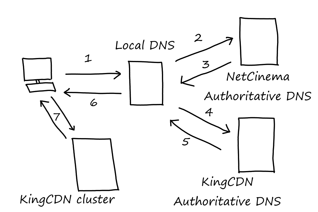
- Our computer sends a DNS query for video.netcinema.com
- The local DNS server contacts an authoritative DNS server for NetCinema.
- The authoritative DNS server sees the word "video" in the hostname and returns a hostname in the KingCDN's domain, e.g., a1105.kingcdn.com
- The local DNS server contacts an authoritative DNS server for KingCDN to get the IP address of a1105.kingcdn.com
- The authoritative DNS server for KingCDN returns the IP address
- The local DNS server sends the IP address back to our browser
- Our browser sets up the TCP connection and plays the video
Notice that our browser doesn't set up the TCP connection with the video company; it sets up the TCP connection with the CDN. The CDN intercepted the request so that it could direct the browser to one of its clusters.
Cluster Selection Strategies
So how do CDNs determine what the best cluster is for a client? One simple way is to pick the cluster that is geographically closest to the client's local DNS. This works most of the time, but sometimes, clusters can be physically close to a client and have a ton of links and routers between them. Also, some clients can use local DNSs located far away from them, so the cluster that's closest to the local DNS isn't close to the client.
The better approach is to do some research. CDNs can perform real-time measurements of delay and performance between clusters and clients by sending pings to local DNSs. This doesn't always work though since local DNSs can be configured to ignore these pings.
Now to the transport layer!
Transport-Layer Services
The transport layer provides logical communication between applications. Logical communication means that, from the application's point of view, it is directly connected to another application. Of course, we know that physically, there are many routers and links between the applications, but logically, it can be seen as one big direct connection. The transport layer abstracts away all the hardware and details to the application layer.
Relationship Between Transport and Network Layers
The transport layer provides logical communication between processes running on different hosts. The network layer provides logical communication between hosts. We'll distinguish the two with an analogy.
Suppose there are two families: one in California and one in New York. These people are old-fashioned and communicate to each other via snail mail. In each family, there is one person responsible for giving the mail to the postal service and giving the mail to the appropriate family member.
Since the postal service moves mail from house to house, the postal service provides logical communication between the two houses. Since the dedicated mail person in each family moves mail from person to person, the dedicated mail people provide logical communication between the families. The postal service is analogous to the network layer and the dedicated mail person is analogous to the transport layer.
The services provided by the transport layer is constrained by the services provided by the network layer. Going back to the analogy, if the postal service takes as long as it wants to deliver mail, then the dedicated mail person can't guarantee how long it will take to receive mail. However, the transport layer can provide some guarantees of its own regardless of whatever happens in the network layer. For example, the transport layer can guarantee reliable data transfer even if the network layer loses or corrupts data.
Overview of the Transport Layer in the Internet
Remember TCP and UDP? These are the two transport-layer protocols provided by the Internet to the application layer. The responsibility of these two protocols is to extend the network layer's delivery service. In other words, once the network layer has done its job delivering data from host to host, it is now the transport layer's job to continue the data delivery to the appropriate process. Extending host-to-host delivery to process-to-process delivery is called transport-layer multiplexing and demultiplexing.
Multiplexing and Demultiplexing
Recall that data in the transport layer are called segments. The process of delivering the segment to the correct socket is called demultiplexing (network layer `rarr` transport layer `rarr` application layer). The process of collecting a message from a socket, encapsulating it into a segment, and sending the segment to the network layer is called multiplexing (application layer `rarr` transport layer `rarr` network layer).
Each socket has a unique identifier (port number) and each segment has a header specifying which socket it needs to go to. Specifically, the header contains the source port number field and the destination port number field. A port number can be any number from 0 to 65535. Ports 0 to 1023 are well-known port numbers and are reserved for common application protocols.
Connectionless Multiplexing and Demultiplexing
Suppose Host A wants to send data to Host B through a UDP connection. The transport layer in Host A creates a segment with the application message, source port number, and destination port number and sends this segment into the network layer. (Multiplexing complete.) The network layer sends it to Host B's network layer, which sends it to Host B's transport layer. The transport layer looks at the destination port number and sends the segment to the appropriate socket. (Demultiplexing complete.)
The transport layer didn't even look at the source port number at any time. So why is that included in the segment header? If Host B wants to send data back to Host A, then it can look at the source port number to know where to send data to.
Connection-Oriented Multiplexing and Demultiplexing
The process is pretty much the same for TCP sockets. In the TCP case, the transport layer looks at the source IP address, source port number, destination IP address, and destination port number to identify the correct socket. This is because TCP is connection-oriented, so it matters where the data is coming from.
In the UDP case, the transport layer only looked at the destination port number (and the destination IP address, which I didn't mention to simplify things) to identify the correct socket.
If two UDP segments have different source ports (or different source IP addresses) and the same destination port (and same IP address), then the two segments will be sent to the same UDP socket.
If two TCP segments have different source ports (or different source IP addresses) and the same destination port (and same IP address), then the two segments will be sent to different TCP sockets.
Connectionless Transport: UDP
UDP is so bare bones that it does about as much as the underlying network layer protocol: IP. Pretty much the only thing it does that IP doesn't do is multiplexing and demultiplexing.
Even though UDP doesn't guarantee reliable data transfer, there are several reasons why an application would want to use UDP:
- They want to bypass TCP's congestion-control mechanism. They don't really care that some data gets lost.
- They want to bypass TCP's handshaking. They want their data to get there as fast as possible.
- They want to support more active clients. UDP doesn't need to maintain connection state.
Even though UDP isn't always reliable, an application using UDP can still have reliable data transfer by adding reliability mechanisms to the application.
UDP Segment Structure
A UDP segment consists of five pieces:
- source port number (`2` bytes)
- destination port number (`2` bytes)
- length (`2` bytes)
- specifies the size of the whole segment (header + application data)
- checksum (`2` bytes)
- application data
| Source Port # | Destination Port # |
| Length | Checksum |
| Application Data | |
UDP Checksum
The checksum is used for error checking. Specifically, the checksum is used to see if any of the bits got messed up while getting transferred.
One's complement is an operation performed on binary numbers. Getting the one's complement of a binary number involves flipping every bit, i.e., `1 rarr 0` and `0 rarr 1`. For example, consider the binary number `1100`. The one's complement of that number is `0011`. This operation is called the one's complement because adding the two numbers together results in a number with all `1`s.
Before sending the segment, UDP has to compute the checksum. It does this by converting the segment into 16-bit numbers, adding all the 16-bit numbers, and performing the one's complement. To simplify things, we will look at 4-bit numbers instead. Suppose a segment is converted into three 4-bit numbers:
`0110`
`0101`
`1010`
The sum of the first two are
`0110`
`0101`
______
`1011`
Now adding this with the third number:
`1011`
`1010`
______
`10101`
There is an overflow here: adding two 4-bit numbers resulted in a 5-bit number. Whenever overflow happens, a "wraparound operation" is applied, where the leftmost bit is taken out and added to the resulting 4-bit number:
`0101`
`1`
______
`0110`
Now we need to get the one's complement of this sum, which is `1001`. `1001` is the checksum of the segment.
When UDP on the receiving end gets the segment, it needs to verify that none of the bits got corrupted. Like the UDP sender, the UDP receiver will also add all the 4-bit numbers together. Adding the three 4-bit numbers (with the wrapround) should result in `0110`. Now, instead of performing the one's complement, the UDP receiver will add this with the checksum in the header, which is `1001`. The result should be `1111`.
In general, if there are no errors, then all the bits will be `1`s*. If there is a `0` somewhere, then UDP knows there is something wrong with this segment. In this case, UDP can either discard the segment or send it to the application with a warning.
*Notice that this is different from saying, "if all the bits are `1`s, then UDP knows that there are no errors."
Principles of Reliable Data Transfer
Here, we'll build out the mechanisms behind a reliable data transfer protocol.
The ideas here apply to a reliable data transfer protocol in general, not just for the transport layer. So the underlying channel doesn't necessarily have to be the network layer (and the layer above doesn't have to be the application layer). Also, instead of "segments", encapsulated data will be generically called "packets".
Suppose our layer is in between an upper layer and a lower layer. Each layer has a channel responsible for sending and receiving data (we'll be building the channel in our layer, so that's why there's no channel for our layer in the drawing). The upper layer calls rdt_send() when it wants to send data into our layer. In our channel is a sender that gets the data and calls udt_send() (the "u" stands for "unreliable") to send the data into the underlying channel. The receiver in our channel gets the data from the underlying channel by calling rdt_rcv() and sends it to the upper layer by calling deliver_data().

Building a Reliable Data Transfer Protocol
A finite-state machine is a model that shows what a machine does on certain actions. A machine starts in a certain state and changes its state as certain events take place.
The dashed arrow points to the initial state of the machine. A solid arrow indicates a transition from one state to another. For every transition, there is a cause and effect. The cause is the event that triggers the transition (think of it as "why is this transition happening?") and the effect is the actions that are taken when the event occurs.
&& is shorthand for "and" and || is shorthand for "or". So "cause: event1 && event2" means that event1 and event2 are causing the transition. And "cause: event1 && (event2 || event3)" means that event1 and either event2 or event3 are causing the transition.
Reliable Data Transfer over a Perfectly Reliable Channel: rdt1.0
First, we'll assume the underlying channel is reliable. This makes things pretty trivial since the underlying channel pretty much did the job for us (the job being reliable data transfer).
On the sender's side:
- take in the data from the upper layer by calling
rdt_send(data) - create a packet by calling
make_pkt(data) - send the packet into the underlying channel by calling
udt_send(packet)
On the receiver's side:
- take in the packet from the underlying channel by calling
rdt_rcv(packet) - extract the data from the packet by calling
extract(packet) - send the data to the receiver by calling
deliver_data(data)

Note there is one FSM for the sender and one FSM for the receiver. Each FSM only has one state because at this point, there's not really much to do besides waiting for data to send or receive. In other words, before we can send data, we have to wait for data. And after we send data, we have to wait for more data. So the only thing to do after taking any action is to wait.
Reliable Data Transfer over a Channel with Bit Errors: rdt2.0
Now let's assume the underlying channel may sometimes corrupt some of the bits. First, we need a way to know if the data is corrupted. The checksum technique is one way, but there are other techniques that are more reliable (see Error-Detection and -Correction Techniques).
Next, we need a way to let the sender know whether the data received is good or bad. For this, we introduce acknowledgments. If the data is good, then the receiver will send a positive acknowledgment (ACK) to the sender. If the data is bad, then the receiver will send a negative acknowledgment (NAK) to the sender, telling the sender to send the data again.
Reliable data transfer protocols based on retransmission are called Automatic Repeat reQuest (ARQ) protocols.
On the sender's side:
- take in the data from the upper layer by calling
rdt_send(data) - create a packet by calling
make_pkt(data) - send the packet into the underlying channel by calling
udt_send(sndpkt) - wait for and get an acknowledgment by calling
rdt_rcv(rcvpkt) - if the acknowledgment is negative, send the packet again by calling
udt_send(sndpkt) - otherwise, if the acknowledgment is positive, get ready to get more data from the upper layer
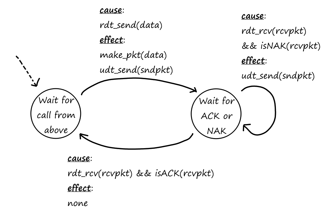
This is the FSM for the rdt2.0 sender.
On the receiver's side:
- take in the packet from the underlying channel by calling
rdt_rcv(rcvpkt) - if the packet is corrupted:
- make a negative acknowledgment by calling
make_pkt(NAK) - send the negative acknowledgment by calling
udt_send(sndpkt)
- make a negative acknowledgment by calling
- otherwise, if the packet is good:
- extract the data from the packet by calling
extract(rcvpkt) - send the data to the receiver by calling
deliver_data(data) - make a positive acknowledgment by calling
make_pkt(ACK) - send the positive acknowledgment by calling
udt_send(sndpkt)
- extract the data from the packet by calling

This is the FSM for the rdt2.0 receiver.
By this design, when the sender is waiting for an ACK or NAK, it cannot get more data from the upper layer. The sender won't send any new data until it knows that the last thing it sent was good. This makes our rdt2.0 protocol a stop-and-wait protocol.
rdt2.1: NACK? What's That?
One thing we haven't considered yet is what if the ACK or NAK is corrupted? After all, an acknowledgment is a packet, so it too can get corrupted. Let's say the receiver sends a NAK, but the NAK gets corrupted. If the sender decides to not do anything, then the receiver never gets any data at all. Consider the other situation where the receiver sends an ACK, but the ACK gets corrupted. If the sender decides to resend the data, then the receiver will get duplicate packets. The problem here is that the receiver doesn't know that this is retransmitted data and will treat this as new data.
The solution is rather simple. If the acknowledgment is corrupted, always resend the data, but add a sequence number to the packet. The receiver can then check the sequence number to see if it's a retransmission. Let's say the sender sends data (with a sequence number) and the data wasn't corrupted. The receiver will send an ACK to the sender, but let's say the ACK gets corrupted. So the sender will resend the data with the same sequence number as before. Seeing that the sequence number of this retransmission is the same as the sequence number of the last packet it received, the receiver will ignore the retransmitted packet.
Since our protocol is a stop-and-wait protocol, alternating between `1`s and `0`s is enough for the sequence number. This is because data gets sent one at a time (because of stop and wait), so as long as the sequence number is different, the receiver will know that it's not a retransmission.
On the sender's side:
- take in the data from the upper layer by calling
rdt_send(data) - create a packet by calling
make_pkt(0, data)- `0` is the sequence number
- send the `0` packet into the underlying channel by calling
udt_send(sndpkt) - wait for and get an acknowledgment by calling
rdt_rcv(rcvpkt) - if the acknowledgment is negative — or corrupted — send the `0` packet again by calling
udt_send(sndpkt) - otherwise, if the acknowledgment is positive, get ready to get more data from the upper layer
- but use sequence `1` for the next packet
- after sending a packet with sequence number `1`, switch back to `0`
- but use sequence `1` for the next packet

This is the FSM for the rdt2.1 sender.
On the receiver's side:
- take in the packet from the underlying channel by calling
rdt_rcv(rcvpkt) - if the sequence number is not `0`, send an ACK, acknowledging the last packet
- check if the packet has sequence number `0` by calling
has_seq0(rcvpkt) - check if the packet has sequence number `1` by calling
has_seq1(rcvpkt)
- check if the packet has sequence number `0` by calling
- if the `0` packet is corrupted:
- make a negative acknowledgment by calling
make_pkt(NAK) - send the negative acknowledgment by calling
udt_send(sndpkt)
- make a negative acknowledgment by calling
- otherwise, if the `0` packet is good:
- extract the data from the packet by calling
extract(rcvpkt) - send the data to the receiver by calling
deliver_data(data) - make a positive acknowledgment by calling
make_pkt(ACK) - send the positive acknowledgment by calling
udt_send(sndpkt)
- extract the data from the packet by calling
- now switch to waiting for a `1` packet
- after getting a `1` packet, switch back to `0`

This is the FSM for the rdt2.1 receiver.
rdt2.2: ACK! ACK! Who's There? Oh, It's You Again
We can get rid of NAKs altogether, so we only have one type of acknowledgment to deal with (I guess having two types is too complicated?). Suppose the sender sends a `0` packet and the receiver gets it just fine, so it sends an ACK back to the sender. Then the sender sends a `1` packet, but that gets corrupted. Instead of sending a NAK for the `1` packet, the receiver can send an ACK for the previous `0` packet. The sender now has received two back-to-back ACK packets (duplicate ACKs) for the `0` packet, so the sender knows that the receiver did not get the `1` packet correctly. In order for this to work, we now have to add the sequence number to the ACK packets as well.
This is like one person asking, "Did you get the message I sent today?" and the other person responding, "The last message I got from you was from yesterday."
On the sender's side:
- take in the data from the upper layer by calling
rdt_send(data) - create a packet by calling
make_pkt(0, data)- `0` is the sequence number
- send the `0` packet into the underlying channel by calling
udt_send(sndpkt) - wait for and get an acknowledgment by calling
rdt_rcv(rcvpkt) - if the acknowledgment is corrupted — or for a `1` packet — send the `0` packet again by calling
udt_send(sndpkt) - otherwise, if the acknowledgment is good and for the `0` packet, get ready to get more data from the upper layer
- but use sequence `1` for the next packet
- after sending a packet with sequence number `1`, switch back to `0`
- but use sequence `1` for the next packet
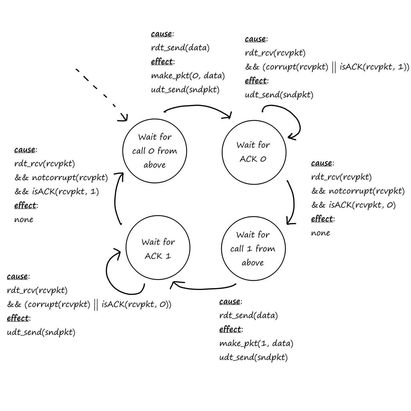
This is the FSM for the rdt2.2 sender.
On the receiver's side:
- take in the packet from the underlying channel by calling
rdt_rcv(rcvpkt) - if the sequence number is not `0` or the packet is corrupted, send an ACK, acknowledging the last packet
- check if the packet has sequence number `0` by calling
has_seq0(rcvpkt) - check if the packet has sequence number `1` by calling
has_seq1(rcvpkt)
- check if the packet has sequence number `0` by calling
- otherwise, if the packet is good and the sequence number is `0`:
- extract the data from the packet by calling
extract(rcvpkt) - send the data to the receiver by calling
deliver_data(data) - make a positive acknowledgment for the `0` packet by calling
make_pkt(0, ACK) - send the positive acknowledgment by calling
udt_send(sndpkt)
- extract the data from the packet by calling
- now switch to waiting for a `1` packet
- after getting a `1` packet, switch back to `0`
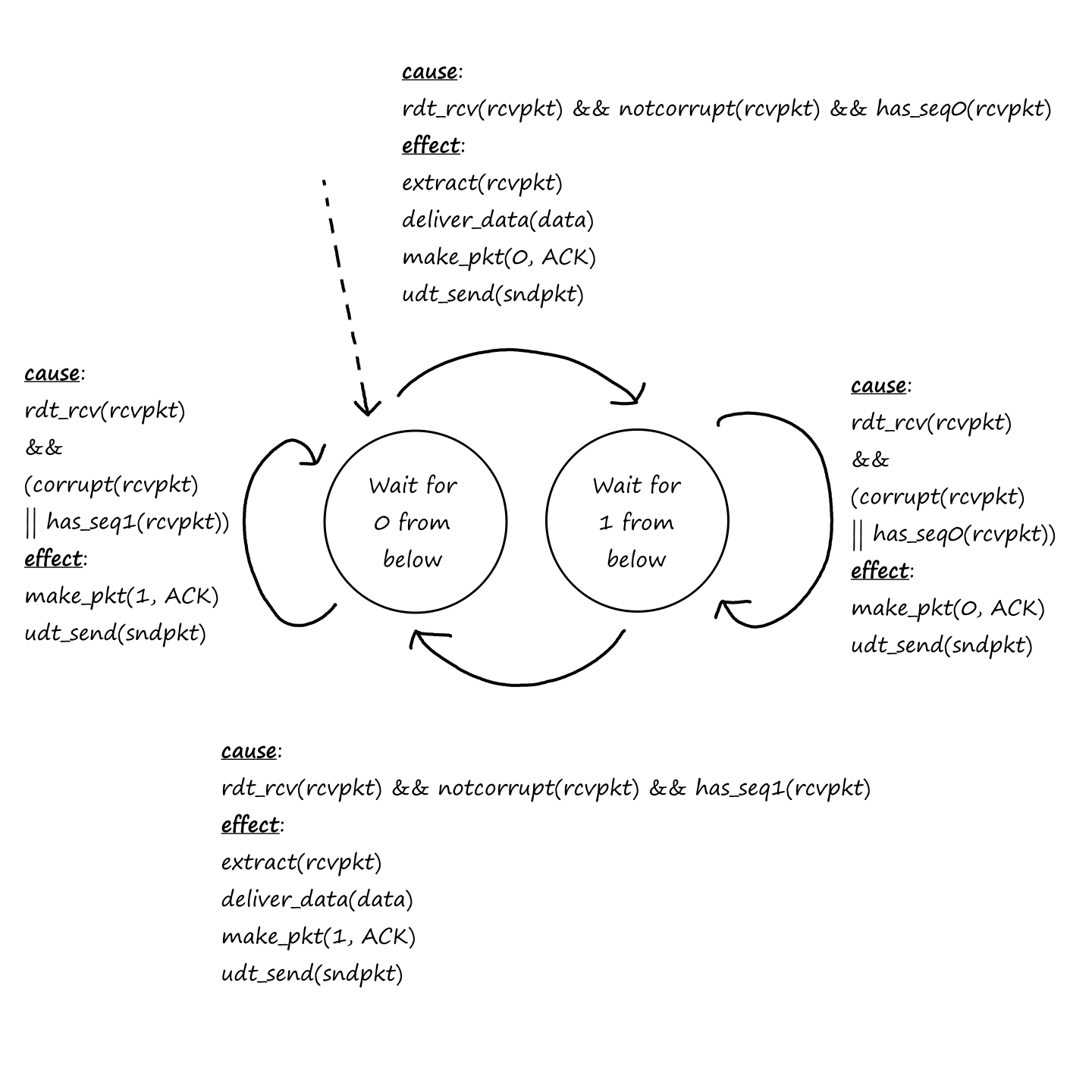
This is the FSM for the rdt2.2 receiver.
Reliable Data Transfer over a Lossy Channel with Bit Errors: rdt3.0
Now let's assume the underlying channel may also lose some packets. Which brings two new problems: how to detect packet loss and how to deal with it. Well, the whole checksum, sequence numbers, ACK packets, and retransmission process already handles how to deal with packet loss. So we just need a way to detect packet loss.
One simple approach is for the sender to resend the packet if no response is ever received. Of course, the sender has to wait for at least some time before assuming the packet (either the packet it sent or the ACK from the receiver) is lost. But how long should the sender wait? At a minimum, it should wait at least as long as the round-trip delay between sender and receiver. However, this is hard to quantify because it includes many variables, including queuing delays and processing delays. At a maximum, packet loss should be handled as soon as possible; it's not good to wait for a long time.
There's not really a perfect solution that can take into account all those variables. The "good enough" solution is for the sender to pick the time it thinks is good enough. One problem (that's not really a problem) is that if the sender doesn't wait long enough, it may end up sending duplicate data packets. But as we saw earlier, the use of sequence numbers allows the receiver to detect duplicates.
In order for this time-based retransmission to work, there needs to be a countdown timer. When the sender sends a packet, it starts the timer for that packet. If the timer goes off before a response is received, then the sender knows to resend the packet (and restart the timer). If a response is received, then the sender will turn off the timer for that packet.
On the sender's side:
- take in the data from the upper layer by calling
rdt_send(data) - create a packet by calling
make_pkt(0, data)- `0` is the sequence number
- send the `0` packet into the underlying channel by calling
udt_send(sndpkt)- start the timer for the `0` packet by calling
start_timer
- start the timer for the `0` packet by calling
- wait for and get an acknowledgment by calling
rdt_rcv(rcvpkt) - if the acknowledgment is corrupted — or for a `1` packet — send the `0` packet again by calling
udt_send(sndpkt) - or if the timer goes off before receiving a response from the receiver, send the `0` packet again
- otherwise, if the acknowledgment is good and for the `0` packet, stop the timer for the `0` packet and get ready to get more data from the upper layer
- but use sequence `1` for the next packet
- after sending a packet with sequence number `1`, switch back to `0`
- but use sequence `1` for the next packet
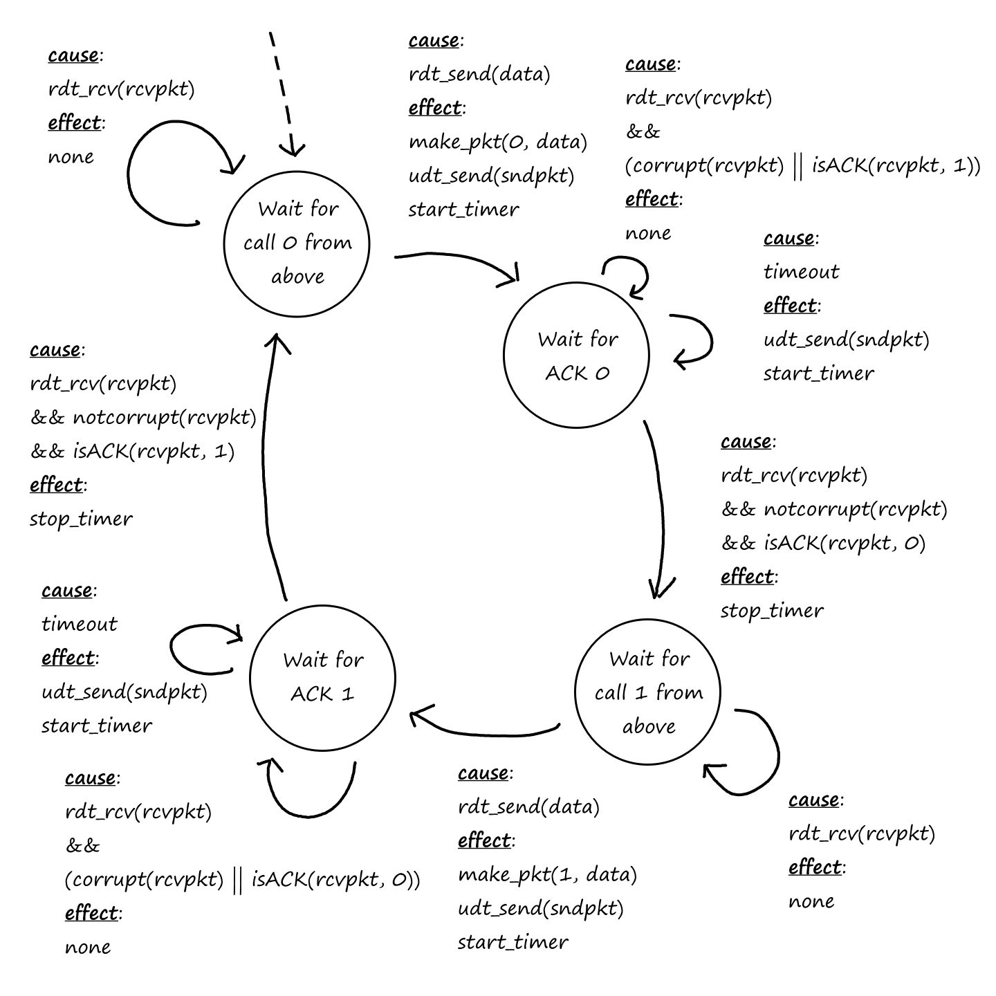
This is the FSM for the rdt3.0 sender.
Notice there's a new self-loop while the sender waits for a call from above. This self-loop is for premature timeouts. Let's say the sender sends a `0` packet and it takes an abnormally long time to reach the receiver. The timer goes off, making the sender think the `0` packet got lost, so the sender sends the `0` packet again. Right after it sends the second `0` packet, the first `0` packet reaches the receiver, so the receiver sends an ACK back to the sender. The sender receives the ACK and goes to waiting for a call from above. While the sender waits for a call from above, the second `0` packet reaches the receiver, so the receiver sends an ACK back to the sender. This is where the self-loop comes in.
On the receiver's side:
- take in the packet from the underlying channel by calling
rdt_rcv(rcvpkt) - if the sequence number is not `0` or the packet is corrupted, send an ACK, acknowledging the last packet
- check if the packet has sequence number `0` by calling
has_seq0(rcvpkt) - check if the packet has sequence number `1` by calling
has_seq1(rcvpkt)
- check if the packet has sequence number `0` by calling
- otherwise, if the packet is good and the sequence number is `0`:
- extract the data from the packet by calling
extract(rcvpkt) - send the data to the receiver by calling
deliver_data(data) - make a positive acknowledgment for the `0` packet by calling
make_pkt(0, ACK) - send the positive acknowledgment by calling
udt_send(sndpkt)
- extract the data from the packet by calling
- now switch to waiting for a `1` packet
- after getting a `1` packet, switch back to `0`
This is the FSM for the rdt2.2rdt3.0 receiver.
Yep, that's right. The receiver for rdt3.0 behaves in exactly the same way as the receiver for rdt2.2. This is because adding a timer just adds more retransmissions. In other words, the receiver will do the same thing (send an ACK) regardless of whether the retransmission was from a timeout or from an error.
Here's how the different scenarios are handled.
No loss:

Lost Packet:
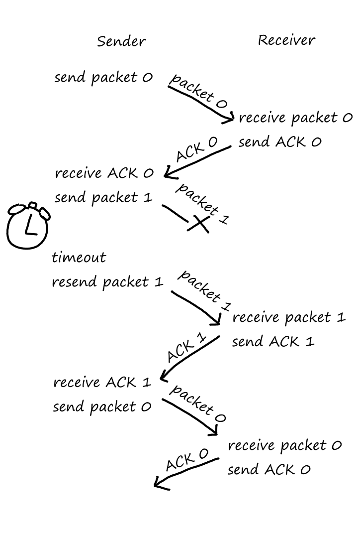
Lost ACK:

Premature timeout:
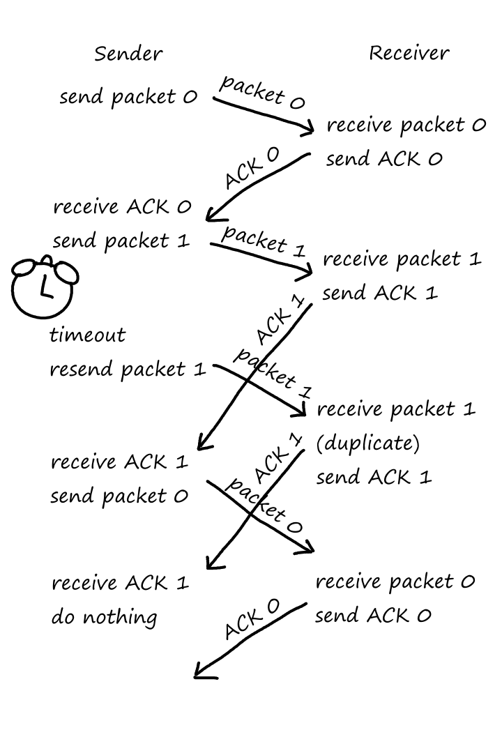
Pipelined Reliable Data Transfer Protocol
While rdt3.0 is a correct protocol, it's not great because of its stop-and-wait nature.
Let's look at the math for sending a packet from sender to receiver. Suppose the RTT is `30` milliseconds; the channel between them has a transmission rate of `1` Gbps (`10^9` bits per second); and the packet size is `1000` bytes (`8000` bits).
The transmission delay is
`d_text(trans)=L/R=(8000text( bits))/(10^9text( bits per second))=0.000008` seconds `=0.008` milliseconds
Once the packet is transmitted, it will take `15` milliseconds to reach the receiver. The receiver now sends the ACK to the sender. For simplicity, we'll assume there is no time to transmit the ACK. It will take `15` milliseconds for the sender to receive the ACK. So this whole process took
`text(RTT)+L/R=30+0.008=30.008` milliseconds
The sender was busy for only `0.008` milliseconds, but the whole process took `30.008` milliseconds. The utilization of the sender (the measure of how busy it was) is
`U_text(sender)=(L/R)/(text(RTT)+L/R)=0.008/30.008~~0.00027`
A low utilization means that it wasn't busy for most of the time, i.e., the sender is being inefficient. In fact, the sender was busy only `0.027%` of the time.
From another point of view, the sender was only able to send `1000` bytes in `30.008` milliseconds. This means the throughput is
`(8000text( bits))/(30.008text( milliseconds))=(8000text( bits))/(0.030008text( seconds))~~267,000` bits per second `=267` kbps.
This is inefficient, considering the fact that the channel between them has a transmission rate of `1` Gbps. (Imagine paying for `1` Gpbs but only getting `267` kbps.)
On top of it all, we haven't even considered processing and queuing delays at intermediate routers in the channel.
It's important to note that all this inefficiency is due to the fact that the sender has to wait for the receiver's response before it can send more data. Naturally, the solution is to let the sender send multiple packets at a time without having to wait for a response. This is called pipelining (because many packets are filling a pipeline). There will be several changes that need to be made for this to work:
- The range of sequence numbers has to be increased. We can't alternate between `0`s and `1`s anymore.
- The sender and receiver need a buffer (queue) to handle multiple packets at a time.
Go-Back-N (GBN)
Let's take a look at the sender's buffer at a random point in time.
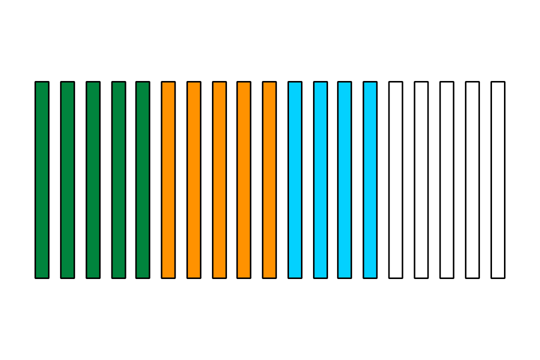
The rectangles are spots in the buffer, where each spot is identified by a sequence number. Green means the packet in this spot has already been sent and ACK'ed. Orange means the packet in this spot has been sent, but no ACK has been received for it yet. Blue means the spot is empty, but once there's a packet in that spot, it will be sent right away. White means the spot is empty and once there's a packet in that spot, it won't be sent right away. (Did you expect me to write that last sentence in white?)
In the Go-Back-N (GBN) protocol, the sender can send multiple packets as long as the number of unacknowledged packets is less than some number `N`. When there are exactly `N` unacknowledged packets in the sender's buffer, the sender is not allowed to send any more data until some of those `N` unACK'ed packets are acknowledged.
To formalize things a bit more, we define base to be the sequence number of the oldest unacknowledged packet and nextseqnum to be the sequence number of the next packet to fill that spot.
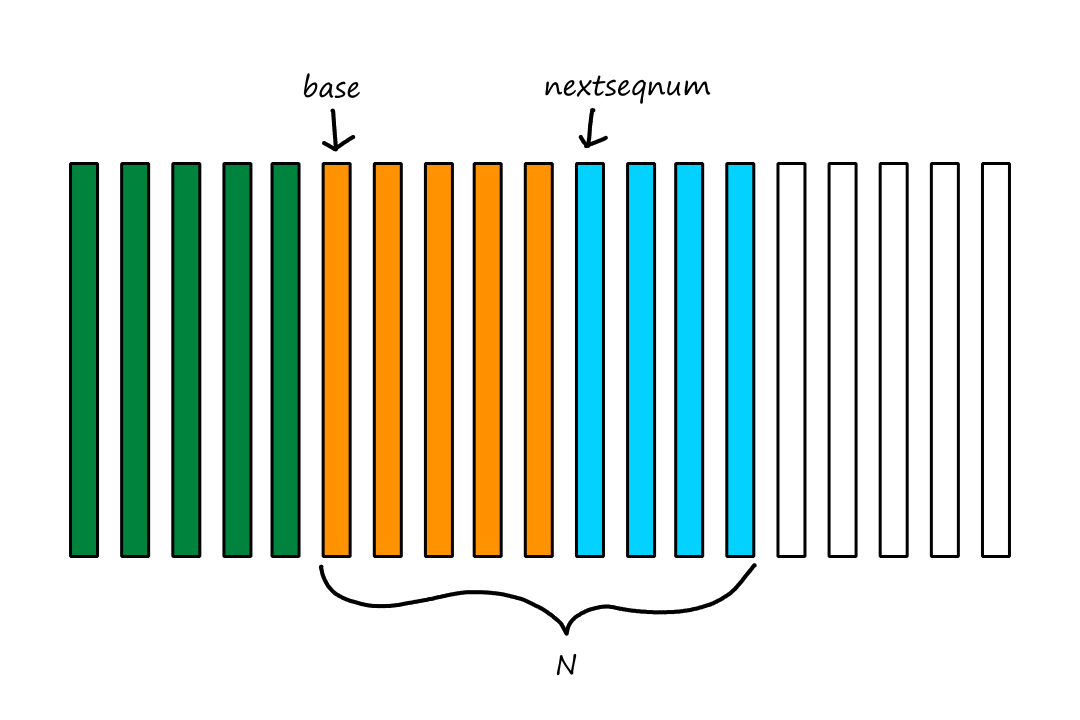
Here's what the buffer looks like as packets get sent, acknowledged, and received:
This sliding animation is why `N` is referred to as the window size and why GBN is a sliding-window protocol.
The sequence number of a packet is stored in the packet's headers, which has limited storage (UDP segments have `8`-byte headers for example). This implies that there's a limit to how high a sequence number can be. Generally, if we devote `k` bits to storing the sequence number, the highest sequence number that can be assigned to a packet is `2^k-1`. Once a packet is assigned the sequence number `2^k-1`, the next packet will be assigned a sequence number of `0`.
For rdt3.0, `k=1`.
When the upper layer has data to send, the sender first checks to see if its window is full, which is the case if there are `N` unACK'ed packets. If it's not full, a packet is created and sent. If it is full, then the packet gets created, but put in the buffer outside the window. (And if the buffer is full, then synchronization methods, like semaphores, are used to control when the upper layer can send data.)
The timer starts when the base packet gets sent. If an ACK is received for the base packet and there are no unACK'ed packets in the window, then the timer is stopped. If an ACK is received for the base packet and there are still unACK'ed packets in the window, then the timer is restarted. In either case, the next packet to be unACK'ed becomes the new base packet.
Now is where we find out why this protocol is called Go-Back-N. If the timer goes off (meaning that the sender thinks a packet got lost), then the sender will resend all packets that are currently unACK'ed. Since there can be at most `N` unACK'ed packets, the sender will go back and send at most `N` packets.
Because the sender sends packets in order, the receiver also expects to get packets in order. It's possible for packets to be out of order if packets get lost.
When the receiver gets a packet with sequence number `n`, the receiver checks if `n` is the expected sequence number, i.e., the receiver checks if the last packet delivered to the upper layer was `n-1`. If it is, then the receiver sends an ACK for packet `n`. If the expected sequence number is not `n`, or the packet got corrupted, then the receiver discards packet `n` and sends an ACK for the last packet it received that was in order.
Since data is delivered to the upper layer one at a time, if packet `k` is received and delivered, then sending an ACK for packet `k` means that packet `k` — and all the packets before `k` — have been received correctly and delivered. This is called cumulative acknowledgment.
There is no need for the receiver to have a buffer. Theoretically, if the receiver is waiting for packet `n`, but it gets `n+1` instead, the receiver could store it in a buffer until packet `n` arrives. But if packet `n` never arrives, both packets `n` and `n+1` will be retransmitted by the sender anyway.
The good thing about not having a buffer to manage is that it reduces complexity. The bad thing about this is that we're throwing away a perfectly good packet. In subsequent retransmissions, that same packet may get lost or corrupted, resulting in more retransmissions.
Suppose the sender's window size is `4`. The sender starts by sending packets `0`, `1`, `2`, and `3`, then waiting for their ACKs. The receiver gets packets `0` and `1`, but let's say packet `2` gets lost. When the sender gets the ACKS for `0` and `1`, the sender sends packets `4` and `5`. The receiver gets packets `3`, `4`, and `5`, but discards them since packet `2` hasn't come yet. (The receiver also sends ACKs for packet `1` since that was the last correctly received packet, but the sender will ignore these since the sender already received an ACK for `1`.)
The timer eventually goes off, so the sender sends packets `2`, `3`, `4`, and `5` again.
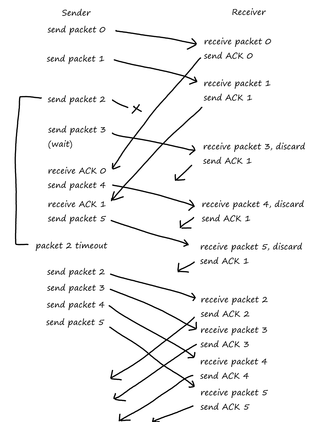
These FSMs are called extended FSMs because there are now variables, like base and nextseqnum, and other programming language constructs.

This is the FSM for the GBN sender.
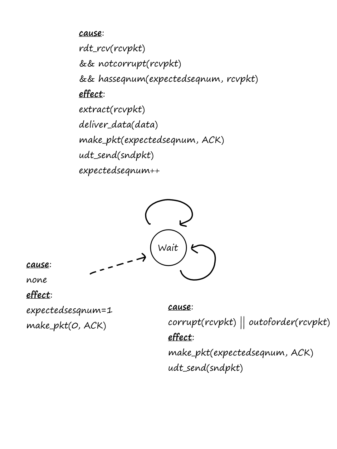
This is the FSM for the GBN receiver.
In the receiver, expectedseqnum is only incremented when a valid packet is received. So when a non-valid packet is received, the receiver sends an ACK for the last correctly received packet, which will have sequence number expectedseqnum.
Selective Repeat (SR)
Even though GBN allows the sender to send multiple packets at a time, there are still some situations where GBN is inefficient. If something goes wrong with just one packet, GBN has to go back `N` and retransmit all those packets again, which is problematic especially if `N` is large.
Based on its name, SR will select only the packets that (it thinks) were lost and retransmit just those packets.

The sender's buffer in SR is similar to the sender's buffer in GBN. But in SR, packets can be ACK'ed out of order.
In order for this to work, the receiver must also have its own buffer.

In this picture, the buffer is not meant to match with the sender's buffer.
Green means the packet in this spot has already been delivered to the upper layer. Red means the packet in this spot has not been received yet. Purple means the packet in this spot has been received and ACK'ed, but not yet delivered to the upper layer. Blue means the spot is empty, but once there's a packet in that spot, it will be ACK'ed. White means the spot is empty and once there's a packet in that spot, it won't be ACK'ed right away. (Hah! I wrote it in white this time!)
In the example above, let's say the sequence numbers of the first two purple packets are `6` and `7`. If packet `5` arrives, then packets `5`, `6`, and `7` will all be delivered to the upper layer at once.
When the upper layer has data to send, the sender first checks to see if its window is full, which is the case if there are `N` packets and at least `1` of them is unACK'ed. If it's not full, a packet is created and sent. If it is full, then the packet gets created, but put in the buffer outside the window. (And if the buffer is full, then synchronization methods, like semaphores, are used to control when the upper layer can send data.)
Since packets are selectively repeated, each packet needs its own timer. (Unlike in GBN where one timer was used for `N` packets.)
If the receiver gets a packet that has already been delivered to the upper layer (sequence number `lt` rcv_base), then the receiver sends an ACK for it and discards it. If the receiver gets a packet outside of its window (sequence number `gt` rcv_base`+N` ), then the receiver puts it in the buffer outside the window. Finally, if the receiver gets a packet with a sequence number inside the window, the receiver sends an ACK for it. And if the sequence number is equal to rcv_base, then it and all consecutive packets that have been ACK'ed will be delivered to the upper layer.
It is necessary for the receiver to send ACKs for packets it has already delivered to the upper layer. Suppose the sender has not received an ACK for the base packet yet, but the receiver has already delivered it to the upper layer. Let's say the ACK from the receiver got lost, so the sender's timer eventually goes off for the base packet, causing the sender to send it again. If the receiver doesn't send an ACK for the base packet it already delivered, then the sender will be stuck forever waiting for the ACK.
Suppose the window size is `4`. The underlined numbers are the sequence numbers in the window. The sender starts by sending packets `0`, `1`, `2`, and `3`, then waiting for their ACKs. The receiver gets packets `0` and `1`, but let's say packet `2` gets lost. When the sender gets the ACKS for `0` and `1`, the sender sends packets `4` and `5`. The receiver gets packets `3`, `4`, and `5`, and buffers them since packet `2` hasn't come yet. The timer eventually goes off for packet `2`, so the sender sends packet `2` again. The receiver gets packet `2` and delivers it along with buffered packets `3`, `4`, and `5` to the upper layer.
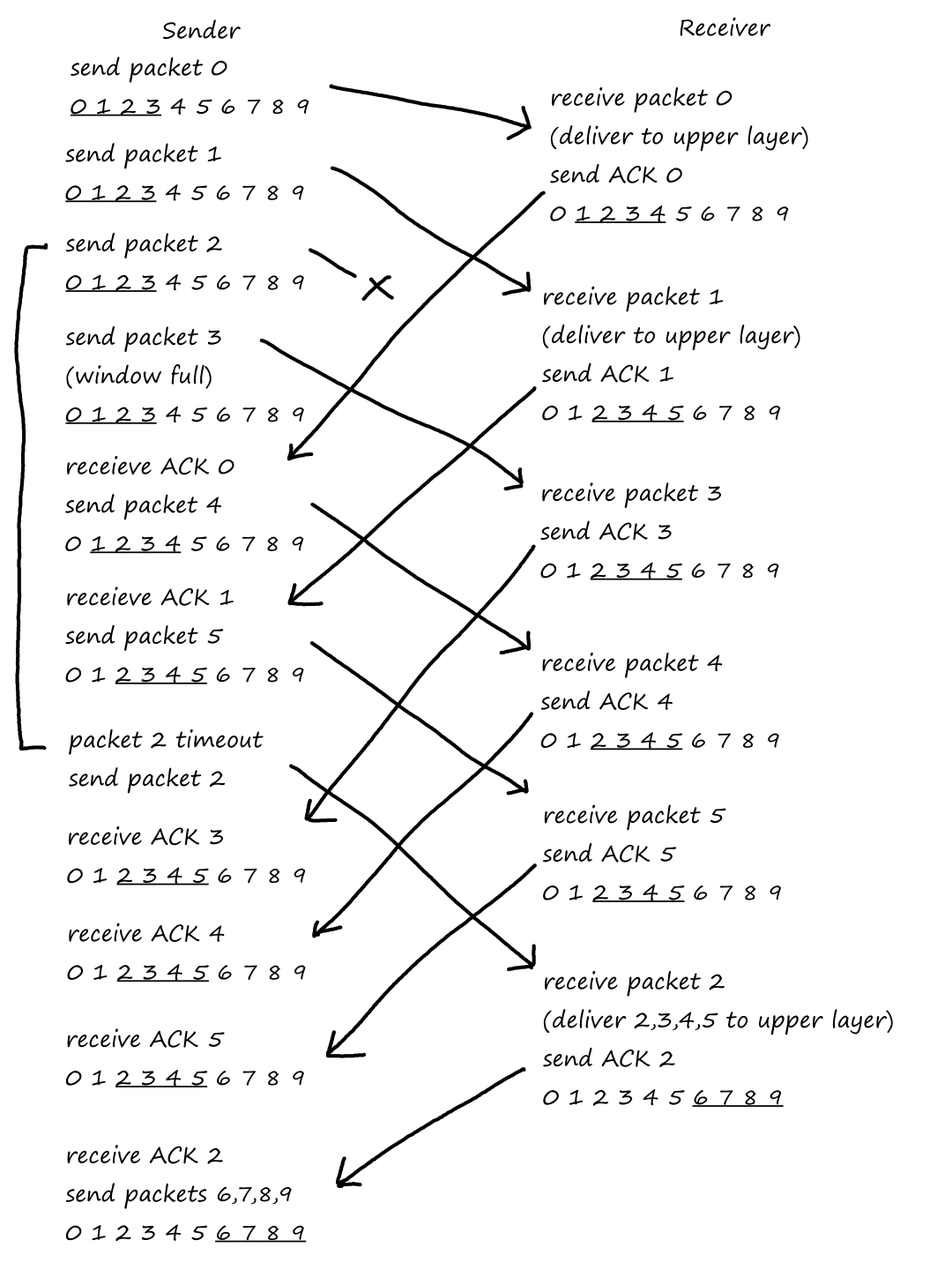
The sender's window does not have to be in sync with the receiver's window. This isn't usually a problem if they sync up eventually. However, it is possible that being out of sync at the wrong time can cause issues, particularly if the size of the window is fairly close to the number of assignable sequence numbers.
For example, suppose the window size is `3` and the number of assignable sequence numbers is `4` (so the assignable sequence numbers are `0`, `1`, `2`, `3`).
The sender starts by sending packets `0`, `1`, and `2`. The receiver gets all of them successfully and the sender gets all their ACKs successfully too. So the sender sends packets `3`, `0`, and `1`. The receiver gets packet `0` correctly, but packet `3` gets lost, so packet `0` on the receiver's side gets buffered.
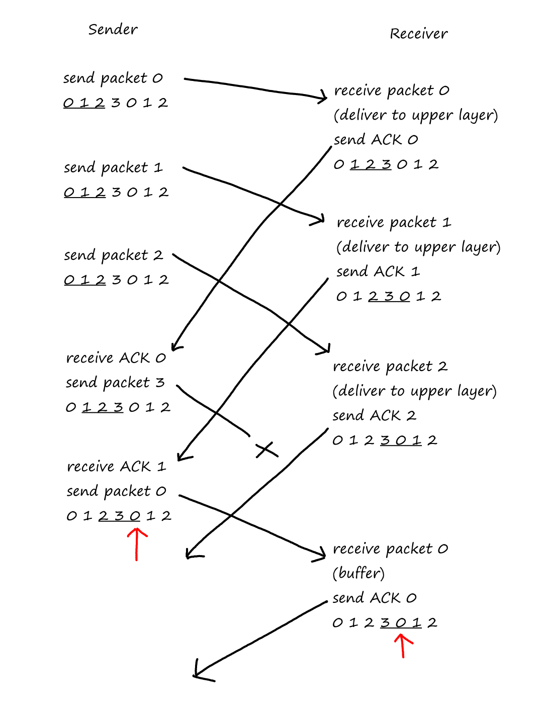
Everything seems normal for now, but let's look at another scenario. Suppose that the ACKs for packets `0`, `1`, and `2` got lost instead. The timer goes off for packet `0`, so the sender resends packet `0`.
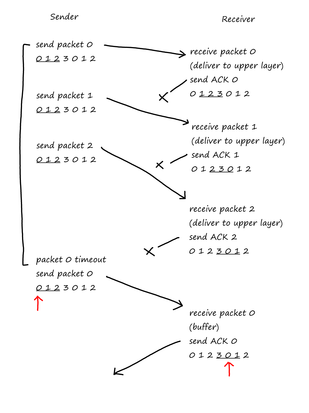
But wait, look at the windows for the sender and receiver! When the sender was sending packet `0` the second time, packet `0` was actually a retransmission. However, the receiver thought it was a new packet `0`.
Furthermore, the receiver thinks everything is fine; and why wouldn't it? From the receiver's point of view, the sequence of events in this situation is exactly the same as the normal one.
In order to avoid this problem of confusing one packet for another, the window size and number of assignable sequence numbers has to be different enough. But how much is enough? (Obviously, different by `1` isn't enough!)
Notice that when the receiver moved by a whole window's length, some of the sequence numbers in the previous window showed up again in the next window.

This is what caused the trouble, because it's possible to get these sequence numbers mixed up with the ones from the previous window (where the other side is stuck on the previous window). Naturally, this means that we should be able to move by a whole window and not see any of the previous sequence numbers. Well, that happens when the number of assignable sequence numbers is (at least) twice the window size.
Here's a table summarizing everything we needed to build a reliable data transfer protocol:
| Mechanism | Description |
|---|---|
| Checksum | Used to detect corrupted packets |
| Acknowledgment | Used to tell the sender that the packet was received correctly |
| Negative acknowledgment | Used to tell the sender that the packet was not received correctly |
| Sequence number | Used to give packets an ordering so the receiver can distinguish duplicate packets and detect lost packets |
| Timer | Used to retransmit lost packets |
| Window, pipelining | Used to allow the sender to send multiple packets at a time, but not too many at once |
Connection-Oriented Transport: TCP
A lot of the stuff we just saw will show up here because, well, TCP is a reliable data transfer protocol.
The TCP Connection
As we've seen several times by this point, TCP is connection-oriented because the two processes communicating with each other have to establish a connection with each other first before any data is sent. What's interesting though (at least to me) is that the lower layers are not aware of "connections"; all they see are packets of data. After all, the handshaking part of TCP (i.e., establishing a connection) is nothing more than packets of data.
TCP provides a full-duplex service, which means that data can go back and forth between Process A and Process B (i.e., data flow is bidirectional)*. A TCP connection is also point-to-point, which means there is only one sender and one receiver at a time. We can't establish a TCP connection between Process A and Process B and have Process C send/receive data to/from them.
*Even though the "Principles of Reliable Data Transfer" section only looked at transferring data from sender to receiver (i.e., unidirectional data transfer), those principles also apply to bidirectional data transfer. In the bidirectional case, there is no longer just one sender and one receiver. There are two hosts that can be sender or receiver depending on who's sending data and who's receiving data at that moment.
Establishing a connection starts with a three-way handshake (animated in "HTTP with Non-Persistent Connections"). After that, the client process sends data through the socket to the transport layer, where TCP puts the data into a send buffer. Then, when it can, TCP gets the data from the send buffer, encapsulates it with headers, and passes it on to the network layer. Eventually, the data reaches the receiver's transport layer, where TCP puts the data into a receive buffer. Finally, the receiver's application process reads from this buffer to get the data.
There is a maximum segment size (MSS) that limits how big a segment can be. This is determined by the maximum transmission unit (MTU), which is the length of the largest link-layer frame that the local sending host is capable of sending. Since a TCP/IP header (a TCP segment encapsulated in an IP datagram) is typically `40` bytes, the MSS is calculated as `text(MSS) = text(MTU) - 40`. From this equation, we can see that MSS is the maximum amount of application-layer data that can be in a segment, not the size of the whole segment. A bit of a misnomer.
TCP Segment Structure
The data portion of the TCP segment contains the application data. If the application data is larger than the MSS, then it is broken up into chunks of size `le` MSS.
The following are included in the TCP segment:
- source (`2` bytes) and destination port (`2` bytes) numbers
- checksum (`2` bytes)
- sequence number (`4` bytes)
- acknowledgment number (`4` bytes)
- receive window (`2` bytes)
- the number of bytes a receiver is willing to accept
- header length (`0.5` bytes)
- flags (`1` byte)
- ACK
- RST
- SYN
- FIN
- CWR
- ECE
- PSH
- if the flag is on, then the receiver should pass the data to the upper layer right away
- URG
- if the flag is on, then (parts of) this data has been marked "urgent" by the sending side
- urgent data pointer (`2` bytes)
- the location of the last byte of urgent data
+-+-+-+-+-+-+-+-+-+-+-+-+-+-+-+-+-+-+-+-+-+-+-+-+-+-+-+-+-+-+-+-+
|          Source Port          |       Destination Port        |
+-+-+-+-+-+-+-+-+-+-+-+-+-+-+-+-+-+-+-+-+-+-+-+-+-+-+-+-+-+-+-+-+
|                        Sequence Number                        |
+-+-+-+-+-+-+-+-+-+-+-+-+-+-+-+-+-+-+-+-+-+-+-+-+-+-+-+-+-+-+-+-+
|                    Acknowledgment Number                      |
+-+-+-+-+-+-+-+-+-+-+-+-+-+-+-+-+-+-+-+-+-+-+-+-+-+-+-+-+-+-+-+-+
| Header |        |C|E|U|A|P|R|S|F|                             |
| Length | Unused |W|C|R|C|S|S|Y|I|       Receive Window        |
|        |        |R|E|G|K|H|T|N|N|                             |
+-+-+-+-+-+-+-+-+-+-+-+-+-+-+-+-+-+-+-+-+-+-+-+-+-+-+-+-+-+-+-+-+
|           Checksum            |      Urgent Data Pointer      |
+-+-+-+-+-+-+-+-+-+-+-+-+-+-+-+-+-+-+-+-+-+-+-+-+-+-+-+-+-+-+-+-+
|                            Options                            |
+-+-+-+-+-+-+-+-+-+-+-+-+-+-+-+-+-+-+-+-+-+-+-+-+-+-+-+-+-+-+-+-+
|                                                               :
:                             Data                              :
:                                                               |
+-+-+-+-+-+-+-+-+-+-+-+-+-+-+-+-+-+-+-+-+-+-+-+-+-+-+-+-+-+-+-+-+
(copied from RFC 9293)
A TCP segment's header is typically `20` bytes.
Sequence Numbers and Acknowledgment Numbers
So far, we've only seen sequence numbers increasing sequentially by `1`. However, TCP works in bytes, not packets.
Suppose a file is being transferred over TCP. Let's say the file size is `500,000` bytes and the MSS is `1000` bytes. This means there will be `(500,000)/1000=500` segments, where each segment is divided into `1000` bytes (numbered starting from `0`*).
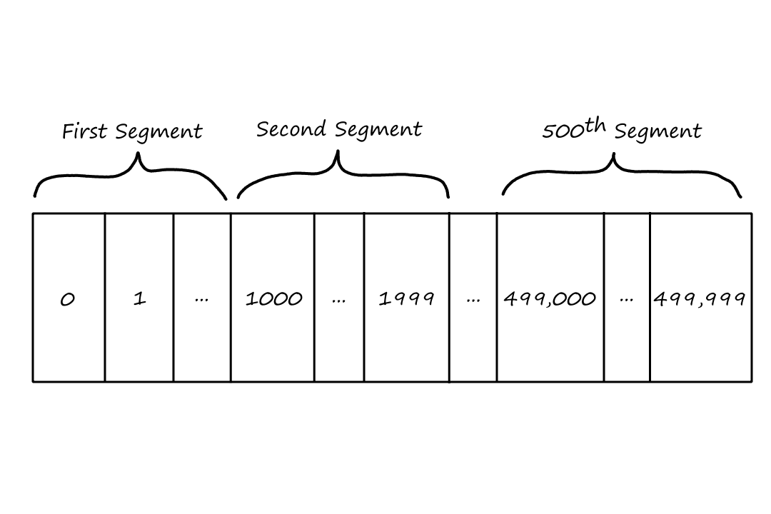
(each rectangle should be the same size but I ran out of room)
The sequence number of the first segment is `0`. The sequence number of the second segment is `1000`. The sequence number of the `500^(th)` segment is `499,000`. Generally, the sequence number for a segment is the byte-stream number of the first byte in that segment.
*For simplicity, we assumed that the initial sequence number starts at `0`. In reality, the initial sequence number is random. This is to prevent the possibility that a segment that is somehow still in the network from a previous connection gets mistaken for a valid segment in a new connection.
The acknowledgment number is the sequence number that the sender is waiting to receive. If the acknowledgment number is `x`, then that means, "I need you to give me a segment with sequence number `x`."
Suppose that Host A has only received bytes `0` through `535` from Host B. On every segment that Host A sends to Host B, Host A will put `536` as the acknowledgment number until Host A gets byte `536` from Host B.
Suppose that Host A has received bytes `0` through `535` and bytes `900` through `1000`. Host A will also put `536` as the acknowledgment number in this case. Notice that Host A received the segments out of order. The TCP RFCs do not specify what to do with out-of-order segments; the decision is left to the people programming the TCP. They can decide to either drop the out-of-order segments or put them in a buffer, which is the preferred method.
Telnet: Sequence and Acknowledgment Numbers in Action
Telnet is an application-layer protocol that allows us to remotely log in to another computer. (It's the unencrypted version of SSH.)
Suppose Host A initiates a Telnet session with Host B (so the person on Host A is remotely logging into Host B). Whenever the user on Host A types something, the input will be sent to Host B, which will send back a copy of the input to Host A. This "echo back" is so the user knows that the remote host received the input. This means that each character travels through the network twice (Host A `rarr` Host B and Host B `rarr` Host A). Let's look at what happens if the user on Host A types a single letter 'C'. (Note that sequence numbers will be increasing by `1` in this case because it only takes `1` byte to store a character.)
Let's say the starting sequence numbers are `42` and `79` for Host A and Host B respectively. When the letter 'C' is typed, Host A sends a segment with sequence number `42` and acknowledgment number `79`. Upon receiving the segment, Host B has to do two things: send an ACK and echo the data back. Both of these can be done in one step. The ACK can be included in the segment by putting `43` as the acknowledgment number. By doing this (a.k.a. piggybacking the acknowledgment), Host B is saying that it is now waiting for byte `43` (implying that it has received `42`). And, of course, echoing the data back is done by putting the data in the segment. Once Host A gets the segment, it sends an ACK back to Host B by sending a segment with acknowledgment number `80`. The sequence number is `43` since Host A last sent `42`, and there is no data since this segment is solely for acknowledgment. So the ACK is not being piggybacked here.
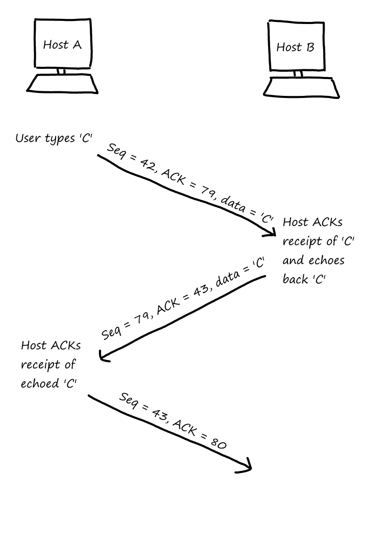
Round-Trip Time Estimation and Timeout
Somewhere in the rdt3.0 section, the question of how long the timeout should be was briefly discussed. In fact, it was mentioned that the timer should be at least as long as the round-trip time between sender and receiver. Now we attempt to quantify that RTT.
Estimating the Round-Trip Time
The round-trip time is the time from when the segment is sent to when the acknowledgment for that segment is received. Let's denote this time as SampleRTT. So every time a segment is sent and acknowledged, the value of SampleRTT changes to however long that segment took.
A SampleRTT is never calculated for a retransmitted segment. This is because if an acknowledgment for that segment came back, it would be hard to tell if the acknowledgment was for the original segment or the retransmitted segment.
The problem is that the RTT can vary wildly from segment to segment, so it's better to keep track of what the average RTT has been. Let's call this average EstimatedRTT. So every time a segment is sent and acknowledged, the average will be updated by:
`text(EstimatedRTT)=(1-alpha)*text(EstimatedRTT)+alpha*text(SampleRTT)`
The recommended value for `alpha` is `0.125`.
(Disclaimer: I hope my math is not wrong!) Suppose we only have one SampleRTT so far; let's call it SampleRTT1. So the EstimatedRTT is just SampleRTT1 at this point*:
`text(EstimatedRTT)=text(SampleRTT)_1`
Now along comes the second SampleRTT.
`text(EstimatedRTT)=(1-alpha)*text(EstimatedRTT)+alpha*text(SampleRTT)_2`
`=(1-alpha)*text(SampleRTT)_1+alpha*text(SampleRTT)_2`
And the third SampleRTT.
`text(EstimatedRTT)=(1-alpha)*text(EstimatedRTT)+alpha*text(SampleRTT)_3`
`=(1-alpha)*((1-alpha)*text(SampleRTT)_1+alpha*text(SampleRTT)_2)+alpha*text(SampleRTT)_3`
`=(1-alpha)^2*text(SampleRTT)_1+(1-alpha)alpha*text(SampleRTT)_2+alpha*text(SampleRTT)_3`
And finally the fourth SampleRTT.
`text(EstimatedRTT)=(1-alpha)*text(EstimatedRTT)+alpha*text(SampleRTT)_4`
`=(1-alpha)*((1-alpha)^2*text(SampleRTT)_1+(1-alpha)alpha*text(SampleRTT)_2+alpha*text(SampleRTT)_3)+alpha*text(SampleRTT)_4`
`=(1-alpha)^3*text(SampleRTT)_1+(1-alpha)^2alpha*text(SampleRTT)_2+(1-alpha)alpha*text(SampleRTT)_3)+alpha*text(SampleRTT)_4`
Generally, after `n` SampleRTTs, the equation looks like:
`text(EstimatedRTT)=(1-alpha)^(n-1)*text(SampleRTT)_1+(1-alpha)^(n-2)alpha*text(SampleRTT)_2+...+(1-alpha)^(n-n)alpha*text(SampleRTT)_n`
`=(1-alpha)^(n-1)*text(SampleRTT)_1+(1-alpha)^(n-2)alpha*text(SampleRTT)_2+...+(1-alpha)^(0)alpha*text(SampleRTT)_n`
`=(1-alpha)^(n-1)*text(SampleRTT)_1+(1-alpha)^(n-2)alpha*text(SampleRTT)_2+...+alpha*text(SampleRTT)_n`
If we let `n rarr oo`, the EstimatedRTT will look like:
`text(EstimatedRTT)=(1-alpha)^(oo-1)*text(SampleRTT)_1+(1-alpha)^(oo-2)alpha*text(SampleRTT)_2+...+alpha*text(SampleRTT)_(n)`
The EstimatedRTT will just converge to `alpha*text(SampleRTT)_n`, which means as we calculate more RTTs, it all eventually just depends on the most recent RTT. But that's boring. Let's look at another interpretation.
Notice that `(oo-1)` is "bigger" than `(oo-2)`. With `(1-alpha)lt1`, this means that the weight applied to SampleRTT1 is "smaller" than the weight applied to SampleRTT2. `(oo-2)` is "bigger" than `(oo-3)`, so the weight applied to SampleRTT2 is "smaller" than the weight applied to SampleRTT3. What we see here is that the older the RTT value is, the less effect it has in determining the value of EstimatedRTT. Which makes sense because newer RTTs are more reflective of the current state of the network. This is why the equation for calculating the EstimatedRTT is called an exponential weighted moving average (EWMA) (the weights are exponentially decreasing).
*According to RFC 6298, the value of EstimatedRTT after one SampleRTT should be SampleRTT.
Setting and Managing the Retransmission Timeout Interval
Okay, so the EstimatedRTT is the average time it takes for a segment to be sent and acknowledged. Since it is the average, there will definitely be segments that take longer than EstimatedRTT. So the timeout should be EstimatedRTT plus some extra length of time. To get a sense of how long some of the segments may take, it is useful to know how varied the RTTs are. Let's call this measure of deviation DevRTT.
`text(DevRTT)=(1-beta)*text(DevRTT)+beta*abs(text(SampleRTT)-text(EstimatedRTT))`
If the SampleRTT is close to EstimatedRTT, then DevRTT will not change by much. But if SampleRTT is much larger/smaller than EstimatedRTT, then DevRTT will change by a lot.
In English, if the RTT is close to the average, then most of the RTTs will be fairly close to each other (i.e., most of them will have roughly the same value). If the RTT is far off from the average, then the range of all possible RTT values will be pretty large.
The recommended value for `beta` is `0.25`.
Now that we know how varied the RTTs can be, we can use that to provide a sort of "safety margin" for those segments that take longer than average.
`text(TimeoutInterval)=text(EstimatedRTT)+4*text(DevRTT)`
The `4` could be because of statistics. To cover `99%` of normally distributed data, we have to add `3` standard deviations to the average (see the 68–95–99.7 rule). So adding `4` standard deviations accounts for `gt 99%`, which means `lt 1%` of segments are expected to timeout prematurely.
Reliable Data Transfer
Now we'll look at how TCP behaves. When there is data from the upper layer, if there is room in the sender's window, the sender encapsulates the data in a segment and passes it to the lower layer. The sequence number is updated by adding to it the length of the data that was just sent.
If the timer hasn't been started yet, then the sender starts the timer as well. This time (pun!), there is only one timer; and that timer is only for the oldest unacknowledged segment. If the timer goes off, then the sender retransmits the segment that timed out and restarts the timer. This differs from GBN, where `N` unacknowledged packets are retransmitted if the timer goes off.
If an ACK is received, the sender looks at the acknowledgment number (let's call it `y`) and compares it with the sequence number of the oldest unacknowledged segment (let's call it base). If the acknowledgment number is greater than base, then that means the receiver successfully received all the segments from base to `y`. So all unacknowledged segments `le y` get marked as acknowledged, and base gets updated to the next oldest unacknowledged segment (which has to be greater than `y`). Also, something new that wasn't in any of the previous protocols is if an ACK is received for any unacknowledged segment, the timer gets restarted.
A Few Examples
In the first example, suppose Host A sends a segment with sequence number `92` and `8` bytes of data. Host B gets the segment and sends an ACK for it, but let's say the ACK gets lost. The timer will go off, so Host A will resend the segment with sequence number `92`. Having already received `92`, Host B will send an ACK for it and discard the segment.

In the second example, suppose Host A sends two consecutive segments. The first segment has sequence number `92` and `8` bytes of data and the second segment has sequence number `100` and `20` bytes of data. Host B gets both of them and sends ACKs for them. The first ACK will have acknowledgment number `100` and the second ACK will have acknowledgment number `120`. But the timer goes off before the ACKs reach Host A. So Host A will retransmit segment `92` and restart the timer.
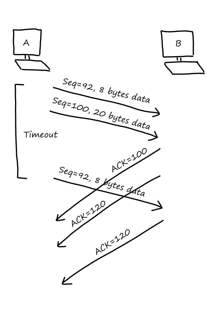
In the third example, suppose that the first ACK gets lost but the second ACK makes it to Host A before the timer goes off. Since ACKs are cumulative, Host A knows that Host B received everything up to `120`, so Host A doesn't need to resend `92` or `100`.

Doubling the Timeout Interval
Whenever there is a timeout, the timeout period is doubled instead of being calculated from EstimatedRTT and DevRTT. So if the timeout interval starts at `0.75` seconds and the timer goes off, the sender retransmits the lost segment and restarts the timer, doubling the timeout interval to `1.5` seconds.
This doubling is only for when timeouts happen. If the timer is started for a different reason (either there is data received from the upper layer or an ACK is received), then the timeout interval is calculated using EstimatedRTT and DevRTT.
This doubling is a form of congestion control. If a segment timed out, it's probably because the network is congested, so doubling the timeout interval is kind of allowing the congestion to clear up before sending more data.
Fast Retransmit
But this doubling introduces a new problem. As more timeouts occur, the timeout interval gets longer and longer as it keeps getting doubled. This is a problem because if a segment gets lost, it will take forever for the segment to be retransmitted. Luckily, there's a way for the sender to know if a segment gets lost before the timer goes off.
Suppose the sender sends segments with sequence numbers `92`, `100`, `120`, `135`, and `141`. Let's say the receiver gets all the segments except `100`. The receiver will send ACKs to the sender with acknowledgment number `100` for all the ACKs. Seeing a bunch of `100`s, the sender can assume that `100` got lost. So before the timer goes off, the sender retransmits segment `100`. This is called fast retransmit.
Fast retransmit only occurs when there are `3` duplicate ACKs for a segment. Fast retransmitting on only `1` duplicate ACK is not a good idea.
Suppose the sender sends segments `92`, `100`, and `120`, and the receiver gets `92`, `120`, and `100` in that order. Upon receiving segment `92`, the receiver will send an ACK with acknowledgment number `100`. Upon receiving segment `120`, the receiver will send an ACK with acknowledgment number `100`. There is `1` duplicate ACK for `100`, but `100` wasn't lost; it just took longer than the other two segments.
However, receiving `3` duplicate ACKs (or any number of duplicate ACKs for that matter) is not a guarantee that there was packet loss. `3` is just an arbitrarily good balance between waiting enough time and not waiting too long.
Go-Back-N or Selective Repeat?
TCP is fairly similar to GBN. There is only one timer for the oldest unacknowledged segment. Out-of-order segments are not individually ACK'ed by the receiver. And there is a base and nextseqnum that the sender keeps track of.
Where they differ. TCP buffers out-of-order segments (sending cumulative ACKs for them) while GBN ignores them (sending ACKs for the last in-order packet it received). If a timeout occurs, TCP will resend only one segment while GBN will resend `N` packets. Sending only one segment on timeout makes TCP similar to SR. The fact that out-of-order segments are buffered also means that the receiver is managing a buffer, similar to SR.
Basicallly, TCP is a combination of GBN and SR.
Flow Control
When the receiver gets and buffers data, the application doesn't necessarily read from this buffer right away. As a result, the receive buffer may get full, which becomes a problem when the sender has more data to send. This can be prevented by TCP's flow-control service, which limits the sender's sending rate to match the application's reading rate.
Flow-control and congestion control are two different things, even though they both limit how much data the sender is sending. Flow-control is to prevent the sender from overwhelming the receiver's buffer while congestion control is to prevent the sender from overwhelming the network.
To simplify things, we'll assume that the TCP receiver discards out-of-order segments instead of buffering them.
In order for the sender to not overwhelm the receiver, the sender needs to know how much space is available in the receiver's buffer. The sender can get an idea of the receiver's buffer size (denoted by RcvBuffer) by maintaining a variable called the receive window (denoted by rwnd), which tracks how much space is available in the buffer.
Suppose Host A is sending a file to Host B. The receiver in Host B will keep track of LastByteRead and LastByteRcvd. LastByteRead is the last byte that the application read from the buffer. LastByteRcvd is the last byte that was placed in the buffer. So for example, things could look like this:
LastByteRead |
LastByteRcvd |
|||
| `9` | `10` | `11` | `12` | `13` |
| empty | contains segment | contains segment | contains segment | empty |
Here, RcvBuffer`=5`, LastByteRead`=9`, LastByteRcvd`=12`. There are `2` empty spots in the buffer, so rwnd`=2`. This can be derived from:
`text(rwnd)=text(RcvBuffer)-(text(LastByteRcvd)-text(LastByteRead))`
There is a "receive window" section in the TCP header; this is where the receiver puts rwnd. So when the receiver sends a segment to the sender, the sender looks at this value to know how much space is available in the receiver's buffer. At the same time, the sender in Host A is keeping track of its own two variables: LastByteSent and LastByteAcked. In order to not overflow the receiver's buffer:
`text(LastByteSent)-text(LastByteAcked)letext(rwnd)`
LastByteSent `-` LastByteAcked is the number of unACK'ed segments on the sender's side. From the sender's point of view, unACK'ed segments are traveling to the receiver. So if there are more unACK'ed segments traveling to the receiver than the receiver's buffer can handle, then obviously the receiver will be overwhelmed.
There is one slight problem though. Suppose the receiver's buffer in Host B gets full. The receiver tells the sender in Host A that its buffer is full so that Host A will stop sending data. Also suppose that Host B has no more data to send to Host A. As the application in Host B is reading data from the receiver's buffer, spots in the buffer start becoming available again. However, since Host B has no more data to send to Host A, the sender in Host A never finds out that the buffer freed up some space.
To get around this, the sender in Host A can occasionally send segments with `1` byte of data so that the receiver in Host B can acknowledge it and respond with its buffer space.
TCP Connection Management
As we've seen before, there is a three-way handshake when establishing a TCP connection. These are the steps involved:
- The client sends a TCP segment to the server. This segment has no data, but the SYN bit is set to `1`. Thus, this segment is called a SYN segment. Also, the segment has a randomly chosen sequence number (called
client_isn). This is the client's way of telling the server what its initial sequence number will be. - The server, seeing the SYN flag set to `1`, prepares all the buffers and variables (all the ones mentioned above) needed for TCP communication. Once this is done, the server sends a TCP segment back to the client, acknowledging the connection request. For the server's ACK segment:
- SYN bit is set to `1`
- acknowledgment number is set to
client_isn`+1` - sequence number is set to a randomly chosen
server_isn
- When the client gets the SYNACK, the client sets up all the buffers and variables too. Then it sends another segment acknowledging the server's connection-granted segment.
- SYN bit is set to `0` since the connection is established
- acknowledgment number is set to
server_isn`+1` - there may be application data if there is data to send
A three-way handshake (as opposed to a two-way handshake) is needed because both sides can send and receive data. Therefore, they need to know each other's sequence numbers and that they are both ready to receive.
In the first step, Host A will tell Host B its sequence number. In the second step, Host B will acknowledge the first step. So now Host B knows Host A's sequence number and Host A knows that Host B is ready to receive. But this only allows for `ArarrB` communication. Host B doesn't know if Host A is ready to receive.
This is why the third step is needed. With Host A acknowledging the second step, Host B can now be sure that Host A is ready to receive, allowing for `AlarrB` communication.
Now let's say the client wants to close the connection. The client will send a segment with the FIN bit set to `1`, telling the server that it wants to close the connection. The server will acknowledge this request by sending an ACK for the segment.
The connection is not closeable at this point though. The client sending the FIN segment only tells the server that it has no more data to send. But the server may still have some data to send to the client. Once the server has no more data to send to the client, the server will send its own FIN segment to the client. When the client receives it and sends an ACK for it, the connection will finally be closed.
The server can also initiate the request to close the connection with the client.
The TCP protocol goes through different TCP states throughout the lifecycle of a connection. For the client, it starts in the CLOSED state and transitions to SYN_SENT when it wants to establish a connection. When it receives a SYNACK from the server, the client moves to the ESTABLISHED state, in which data is transferred back and forth. When the client wants to close the connection, it transitions to FIN_WAIT_1, where it waits for the server to acknowledge the close request. Once the server acknowledges it, the client moves to FIN_WAIT_2, where the client waits for the server to send the FIN segment. After getting the FIN segment from the server, the client sends an ACK for it and moves to TIME_WAIT. The connection is not closed yet; the client waits for a specified time in case it needs to resend the ACK. After the wait, the connection is closed.

For the server, most of the states seem pretty self-explanatory. The CLOSE_WAIT state handles the situation where the client wants to close the connection but the server still has data to send to the client. More generally, the wait is there so that any delayed segments (either still in the network or waiting to be sent by the server) can be handled.
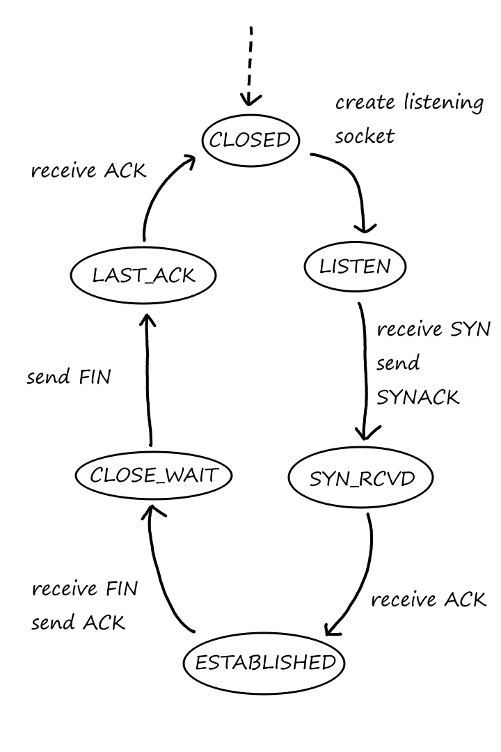
If the client attempts to establish a connection to a non-valid port, the server will send a reset segment to the client. The reset segment has the RST flag set to `1`.
The SYN Flood Attack
As we saw earlier, when the client sends a SYN segment to the server in the first step of the handshake, the server prepares all the resources needed for the connection. Essentially, the server reserves those resources until the connection is established.
Attackers can take advantage of this by sending a bunch (emphasis on a bunch) of SYN segments to the server and never completing the third step of the handshake. Not completing the handshake is the important part because this makes the server reserve a bunch of resources for connections that will never be established. Then, when legitimate clients want to establish a connection to the server, the server denies these requests because there are no more resources available — they were all reserved for the attackers who never plan on using those connections. This is a form of Denial of Service (DoS) attack. The server is forced to deny its service to everyone because of an attack.
It may be obvious that when the server gets a SYN segment, it shouldn't immediately start reserving resources. In fact, the resources should only be allocated after the third step of the handshake is complete, i.e., after the client sends the ACK. But if the server is no longer maintaining any resources (like who wanted to connect in the first place), how would the server know that an ACK is from a client who sent the SYN segment earlier? This is where SYN cookies come in.
When the server gets a SYN segment, it looks at the segment's source IP, source port, destination IP, and destination port. It uses all those numbers, along with a secret number, to create a special number that encodes all that information in a secure way. This value is the SYN cookie. This value is also the server's initial sequence number. So when the server sends the SYNACK in step 2 of the handshake, that SYNACK will have sequence number equal to the SYN cookie.
If the client completes the third part of the handshake, it will send an ACK to the server. This ACK will have the SYN cookie `+1` as the acknowledgment number. When the server gets the ACK, the server performs the same operations it did the first time by using the ACK segment's source IP, source port, destination IP, destination port, and the server's secret number. If this generated number `+1` matches the acknowledgment number of the client's ACK, then the server knows that this ACK was for the SYN sent earlier.
If the client doesn't complete the third part of the handshake, no harm is done because no resources were allocated.
The server's secret number is an important part in generating the SYN cookie. IP addresses and port numbers are obtainable information, so anyone could generate the SYN cookie and send fake ACKs. Only the server knows the secret number, so only the server can tell whether the SYN cookie is real or fake.
TCP Congestion Control
Network congestion is caused by too many senders sending data at a rate that is too fast for the network to handle. This can lead to packet delays and packet loss. To try and prevent this, TCP uses something called end-to-end congestion control. This means that congestion is detected by the presence of packet loss and delays.
The other approach for congestion control is network-assisted congestion control. This means that congestion is detected by the network routers telling us (the transport layer) that there is congestion.
Classic TCP Congestion Control
The sender will control its send rate based on how much congestion is in the network. If there is little to no congestion, then the sender will increase its send rate. If there is congestion, then the sender will slow down its send rate. So, how do we control the sender's sending rate?
Earlier, we saw that the sender keeps track of LastByteSent, LastByteAcked, and rwnd. For congestion control, the sender keeps track of one more variable called the congestion window (denoted by cwnd). This congestion window is an arbitrary dynamic value that is used to limit the sender's rate. So now, the number of unACK'ed segments on the sender's side cannot exceed the receiver's free buffer spaces and the congestion window (whichever one is lower):
`text(LastByteSent)-text(LastByteAcked)le min{text(cwnd),text(rwnd)}`
To only focus on congestion control, we'll ignore rwnd for the rest of the section. If the sender has data to send, then it will be able to send cwnd bytes of data. After one RTT, the sender will receive ACKs for those bytes. Ignoring loss and packet delays, the sender is roughly sending data at a rate of `(text(cwnd))/(text(RTT))` bytes per second. So by adjusting the value of cwnd, we can control the sender's sending rate.
For example, if cwnd`=500` bytes and one RTT is `200` milliseconds, then the sender's sending rate is
`(text(cwnd))/(text(RTT))=(500text( bytes))/(200text( ms))=(500text( bytes))/(0.2text( seconds))=(2500text( bytes))/(1text( second))=2.5text( kilobytes/sec)`
One subtle note about the interpretation of RTT: instead of being the round-trip time for a single segment, RTT will be referring to the round-trip time for sending cwnd bytes.
How can we (the sender) tell if there is congestion? Well, if there is a lot of congestion, then it's likely that packets will be dropped. We know packets are dropped (or considered dropped), when the timer goes off or three duplicate ACKs are received (see the Fast Retransmit section). So if there is a loss event, then the sender's sending rate should be lowered.
If there is not a lot of congestion, then the sender will receive ACKs, in which case the sender's sending rate can be increased. However, there could be a middle-ground situation where there is not too much congestion, but there is still a fair amount of it. In this case, the ACKs will come back, just at a slower rate. This is an indication that the sender's sending rate can be increased, just not by too much. Since TCP uses acknowledgments to trigger (or clock) an increase in congestion window size, TCP is self-clocking.
All of these points lead to this strategy: if ACKs keep coming, keep on increasing the sending rate until no more ACKs come. If no more ACKs come, then decrease the sending rate to a point where ACKs will come and start increasing the rate again.
So we know when the sending rate should be changed, but now the question is by how much? There is a TCP congestion-control algorithm that decides.
Slow Start
At the beginning of the TCP connection, cwnd is initialized to `1` MSS, and every time an ACK is received, cwnd is increased by `1`. So the sender starts by sending `1` segment, then `2` segments, then `4` segments, then `8` segments, and so on. As we can see, the sending rate is doubled, causing it to grow exponentially. This process is called slow start.
If there is a timeout, then cwnd will be reset to `1` and start doubling again. However, we know that we will eventually get a timeout again by repeating the same process. To prevent this, we keep track of what cwnd was when the timeout occurred and stop slow start before it reaches that point. The "slow start threshold" (denoted as ssthresh) is set to half of whatever cwnd was when the timeout occurred. So slow start will keep doubling cwnd until its value is equal to ssthresh.
Congestion Avoidance
Now the value of cwnd is ssthresh. Since we're at a point where congestion could occur, the sending rate should be increased slowly. So rather than doubling cwnd, it will be increased by just `1` MSS instead. For example, if the MSS is `1000` bytes and cwnd is `10,000` bytes, then one RTT consists of `10` segments. After ACKs have been received for those `10` segments, the cwnd will be `10,000+1000=11,000` bytes.
This is equivalent to increasing cwnd by `text(MSS)/(text(cwnd)/text(MSS))=text(MSS)*(text(MSS)/text(cwnd))` on every ACK. `text(cwnd)/text(MSS)` is the number of segments that can be sent, which in turn, is the number of ACKs that will be received. So increasing cwnd by `text(MSS)/(text(cwnd)/text(MSS))` on every ACK will result in an increase of `1` MSS on all ACKs.
For the above example, cwnd will be increased by `1000/((10,000)/1000)=100` bytes on every ACK. Since there are `10` ACKs in one RTT, cwnd will be increased by `100*10=1000` bytes `=1` MSS on all ACKs.
Even though we're increasing the sending rate cautiously, we will still eventually raise it to the point where there's a timeout. When that happens, ssthresh gets updated to half of whatever cwnd was when the timeout occurred and cwnd gets reset to `1`. Yeah, the same procedure as in slow start.
Fast Recovery
So far, we've only seen what happens when congestion is detected by a timeout. As we established earlier, packet loss, and thus congestion, can also be detected by triple duplicate ACKs. This type of congestion is not as bad though, because at least the ACKs were able to make it through. So the sending rate doesn't need to be decreased as much. cwnd is essentially* halved, and ssthresh gets updated to half of whatever cwnd was when the triple duplicate ACK occurred.
*Technically, cwnd is halved `+3` (to account for the triple duplicate ACKS). ssthresh is still half of cwnd though (before the `+3`).
Now cwnd is increased by `1` MSS for every duplicate ACK that caused TCP to enter the fast recovery stage. If the ACK for the missing segment comes, then TCP goes back to congestion avoidance. But if a timeout occurs, then TCP goes back to slow start. Note that cwnd is not changing as new segments are sent and ACK'ed (it only changes on duplicate ACKs).
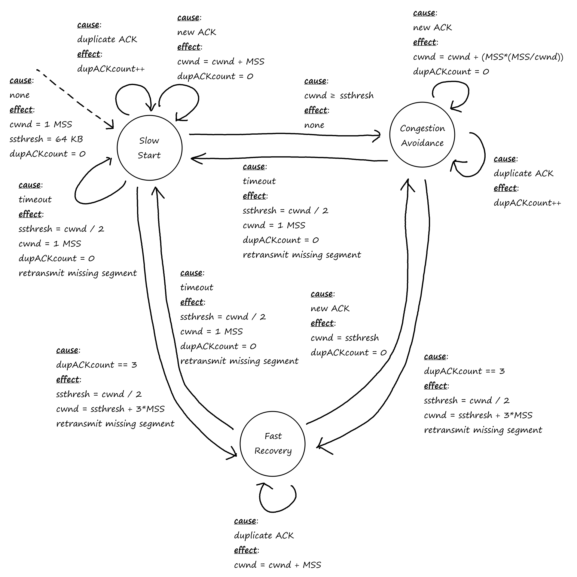
Slow start and congestion avoidance are required for TCP, but fast start is only recommended. TCP Tahoe is an early version of TCP that only has slow start and congestion avoidance, so every time packet loss is detected, TCP switches to slow start regardless of whether it was a timeout or triple duplicate ACK. TCP Reno, a newer version of TCP, includes fast recovery.
The graph shows the changes to cwnd under TCP Reno in a hypothetical transmission scenario.
What are the intervals of time when TCP slow start is operating?
[1, 6] and [23, 26] because the congestion window size is doubling in these intervals
What are the intervals of time when TCP congestion avoidance is operating?
[6, 16] and [17, 22] because the congestion window size is increasing by `1` in these intervals
After the 16th transmission round, is segment loss detected by a triple duplicate ACK or by a timeout?
triple duplicate ACK because the congestion window size is halved`+3`
(the easier way to tell is to see that the congestion window size is not dropped to `1`)
After the 22nd transmission round, is segment loss detected by a triple duplicate ACK or by a timeout?
timeout because the congestion window size is dropped to `1`
What is the initial value of ssthresh at the first transmission round?
32 because that's when slow start stops and congestion avoidance begins
What is the value of ssthresh at the 18th transmission round?
21 because ssthresh gets set to half of whatever cwnd was when packet loss was detected, which was 42
What is the value of ssthresh at the 24th transmission round?
14 because ssthresh gets set to half of whatever cwnd was when packet loss was detected, which was 29
During what transmission round is the 70th segment sent?
7
packet 1 is sent in round 1 (cwnd = 1)
packets 2-3 are sent in round 2 (cwnd = 2)
packets 4-7 are sent in round 3 (cwnd = 4)
packets 8-15 are sent in round 4 (cwnd = 8)
packets 16-31 are sent in round 5 (cwnd = 16)
packets 32-63 are sent in round 6 (cwnd = 32)
packets 64-96 are sent in round 7 (cwnd = 33)
Assuming a packet loss is detected after the 26th round by the receipt of a triple duplicate ACK, what will be the values of the cwnd and ssthresh?
cwnd = 7 and ssthresh = 4
when packet loss is detected, cwnd = 8, so by the rules of fast recovery, ssthresh gets set to half of cwnd and cwnd gets set to half + 3
TCP Congestion Control: Retrospective
Since the congestion window grows exponentially during slow start, TCP doesn't remain in slow start for very long. So most of the changes to the congestion window size are adding `1` and dividing by `2`. Because of this, TCP congestion control is referred to as additive-increase, multiplicative decrease.
This is assuming that most/all packet losses are detected by triple duplicate ACKs rather than timeouts. Although one could argue that setting the congestion window size to `1` is a multiplicative decrease (a division by cwnd 😏).
Macroscopic Description of TCP Reno Throughput
Let `w` be the current window size at any given time. Let `W` be the window size when a loss event occurs.
If it takes one RTT to get ACKs for `w` bytes, then the sending rate is about `w/text(RTT)`. This rate keeps increasing by `1` MSS until it reaches `W/text(RTT)` when a loss event occurs. Then the rate drops to `W/text(RTT)*1/2=W/(2text(RTT))` in response to the loss event and increases by `1` again. And this repeats over and over again.
Assuming the values of `W` and RTT stay mostly consistent the whole time, the sending rate increases between `W/text(RTT)` and `W/(2text(RTT))`. So the average throughput is
`(W/text(RTT)+W/(2text(RTT)))/2=((2W)/(2text(RTT))+W/(2text(RTT)))/2=((3W)/(2text(RTT)))/2=(3W)/(4text(RTT))=(0.75W)/text(RTT)`
Other TCP Variations
Explicit Congestion Notification (ECN)
Even though TCP uses end-to-end congestion control, there have been some proposals to include network-assisted congestion control, in which the routers in the network layer explicitly say there is congestion. This involves carrying the information in two bits of the datagram's header field.
If a router is experiencing congestion, then it will set one of the ECN bits to `1`. At the transport layer, if the TCP receiver sees that this bit is on, it will set the ECE bit to `1` in the ACK segment's header field, so that the TCP sender knows that there is congestion. ECE stands for "Explicit Congestion Notification Echo", so the receiver is "echoing" the news from the network layer that there's congestion.
Seeing the ECE bit on, the TCP sender halves the congestion window (just like it would if there was actual packet loss) and sets the CWR (Congestion Window Reduced) bit in the header of the next transmitted segment to let the receiver know that it has reduced its window size. If the sender doesn't tell the receiver, then the receiver will think that the sender hasn't reduced its window size yet, so it will keep including the ECE bit, which in turn will force the sender to keep halving its window size.
The definition of congestion at the router level is not explicitly defined; it's up to the router vendor and network operator to work out what congestion means.
One idea is that turning the bit on can mean that congestion is close to happening. Maybe the router's buffers are close to being full. This proactive detection is the opposite of end-to-end network congestion's reactive detection where congestion is detected after packet loss has already occurred.
So one of the ECN bits is turned on by the router if it experiences congestion. The other ECN bit is used to let the routers know that the TCP sender and receiver are ECN-capable, that is, they know what to do if there is ECN-indicated network congestion.
Delay-based Congestion Control
Another proactive approach to detecting congestion is to measure every RTT. Let's say the sender knows what the RTT is when there's no congestion at all (of course, this RTT would be relatively low). If most of the RTTs are close to that value, then the sender knows there isn't congestion. But if the RTTs start to become a lot larger than the uncongested RTT, then the sender knows that congestion is coming.
The RTT when there's no congestion at all can be denoted as `text(RTT)_text(min)`. Then the uncongested throughput is `text(cwnd)/text(RTT)_text(min)`. If the current actual throughput is close to this value, then the sending rate can be increased since there's no congestion. But if the current actual throughput is much lower than this, then the sending rate should be decreased since there is congestion.
TCP Vegas uses this approach.
Fairness
For a congestion-control mechanism to be fair, all connections should be able to achieve approximately equal transmission rates. If there are `K` TCP connections all passing through a bottleneck link with transmission rate `R`, then each connection's average transmission rate should be `R/K`, i.e., each connection should get an equal share of the link bandwidth.
Suppose there are only `2` TCP connections sharing a single link with transmission rate `R`. To see if TCP's congestion control is fair, we could plot each connection's (hypothetical) throughputs throughout the duration of the connection. The full bandwidth utilization line marks the points where the link is at full capacity, which means the combined throughput is `R`. Note that if the combined throughput exceeds `R`, then there will be packet loss (since there will be more packets than the link can handle). The equal bandwidth share line marks the points where both of the connection's throughputs are equal to each other.
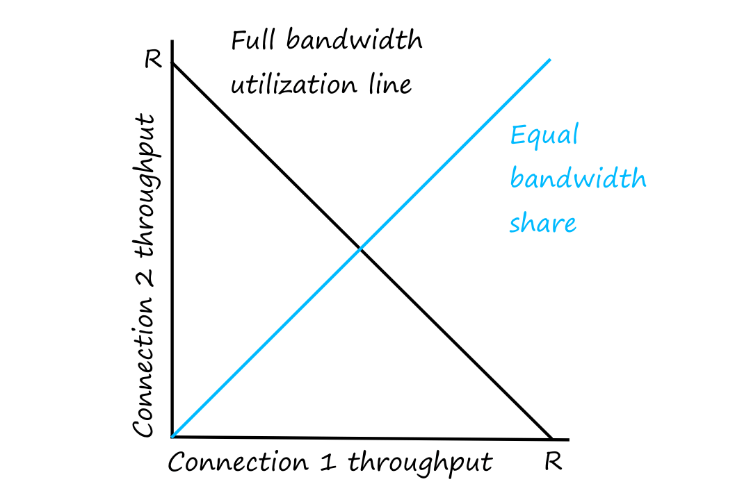
Their throughput should be on the full bandwidth utilization line so that the link is maximally utilized. However, to be fair, one connection shouldn't have much more throughput than the other. Ideally, their throughput should be in the middle of everything.
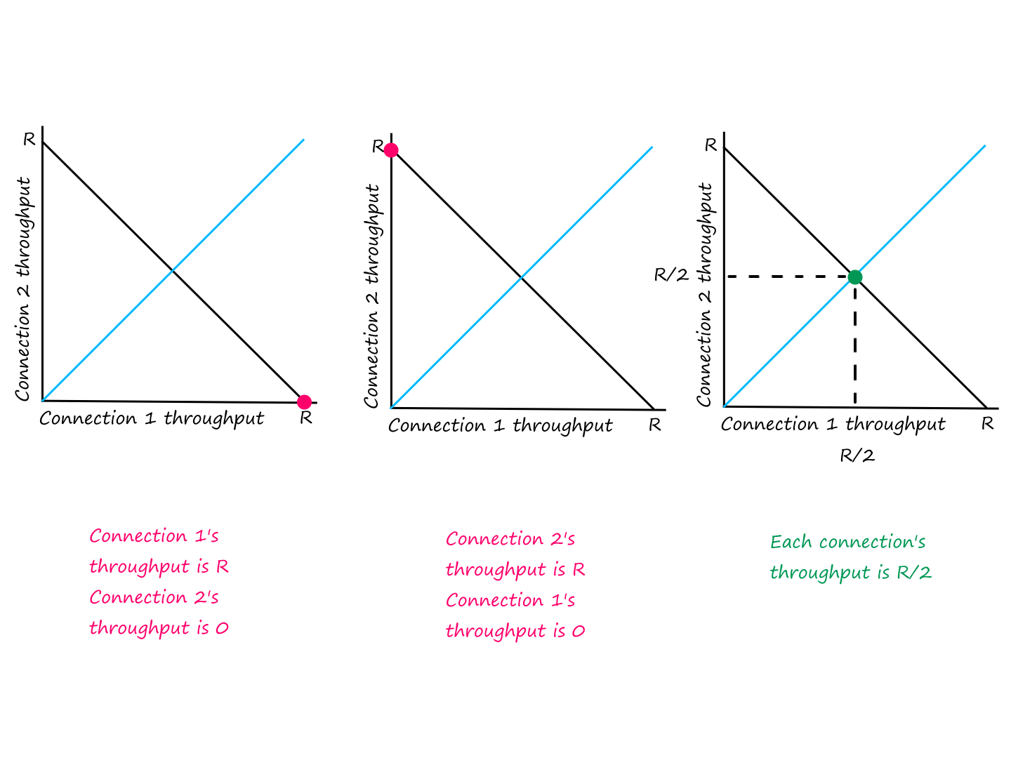
- Let's say both of their throughputs start at point A. Since their throughputs are `lt R`, both connections will continuously increase their window sizes by `+1`.
- Eventually, their throughputs will be `gt R`, so there will be packet loss soon. Suppose that happens at point B.
- In response to congestion, both connections will halve their windows (to point C).
- Since their throughputs are `lt R`, both connections will continuously increase their window sizes by `+1`.
- Eventually, their throughputs will be `gt R`, so there will be packet loss again. Suppose that happens at point D.
- In response to congestion, both connections will halve their windows (to point E).
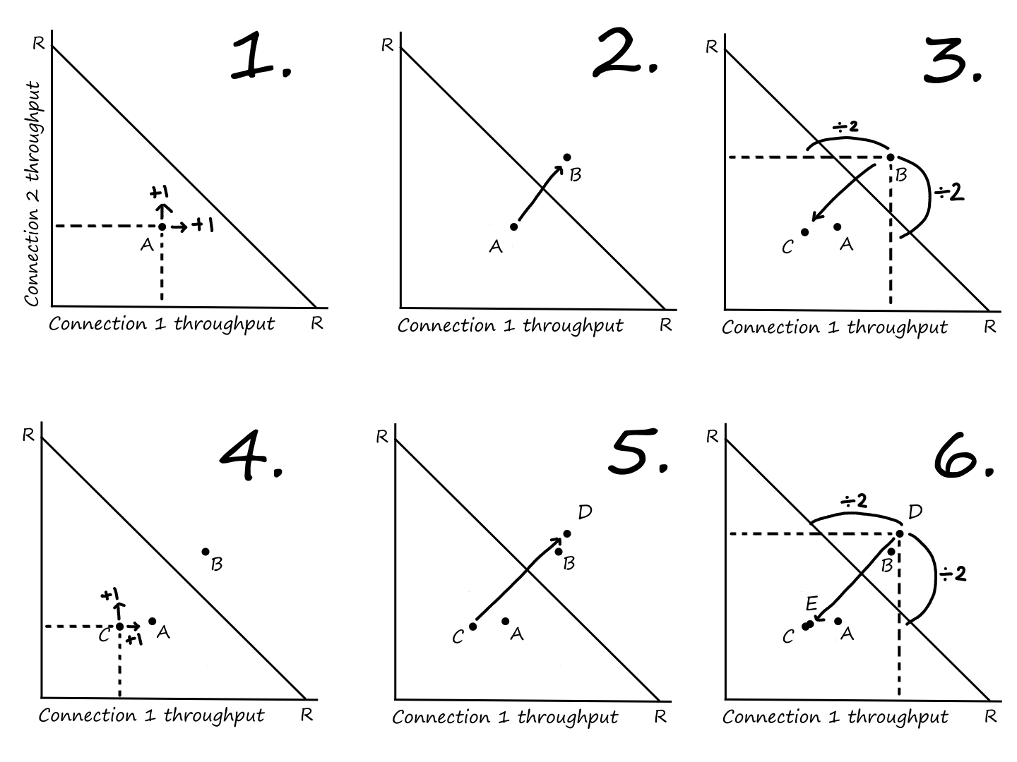
Notice that both throughputs eventually end up along the middle, where the equal bandwidth share line should be. Since both connections are achieving an equal amount of throughput, things are fair.
Once their throughputs are along the equal bandwidth share line, they will continue going back and forth along that line. By definition, the equal bandwidth share line is on the line `y=x`. Once their throughputs are on that line, their throughputs are equal to each other. So performing the same operations (`+1`, `-:2`) on the same numbers still keeps the numbers equal to each other. And since they're equal, they belong on the line `y=x`, which is the equal bandwidth share line.
Also, their throughputs will converge to the middle regardless of where their initial throughputs are. It's sorta like dividing two even numbers by `2`, where one number may be larger than the other. Eventually, they both end up at `1`.
Several assumptions were made for the above hypothetical scenario:
- each connection has a large amount of data to send
- there is no UDP traffic passing through the link
- the two connections have the same MSS and RTT
- they are in congestion avoidance mode at all times
While these conditions are almost never true, the above idea about why TCP is fair is still true.
Fairness and UDP
UDP doesn't have a congestion-control mechanism; it will just keep pushing data into the network. As a result, UDP traffic can theoretically force out TCP traffic. This isn't fair! But there are some mechanisms in place to prevent this from happening.
Fairness and Parallel TCP Connections
As we've seen before, applications can open multiple parallel TCP connections. This can cause an application to unfairly get more of the available bandwidth.
Suppose there are `9` applications that are each using only `1` TCP connection over a shared link with transmission rate `R`. So each application has a transmission rate of `R/9`. Now along comes another application, but this one opens `11` parallel TCP connections. Each connection will now have a transmission rate of `R/20`, but one of the applications owns `11` of those connections, so that application is using more than half of the available bandwidth.
Now to the network layer!
Overview of Network Layer
The network layer is responsible for transferring the transport layer's segment from router to router in the network core. So the network layer is implemented in end systems and routers (whereas the application and transport layer only existed in the end systems).
The network layer can be divided into two parts: the data plane and the control plane. The data plane is responsible for forwarding a datagram from a router's input link to its output link. The control plane is responsible for routing a datagram from source to destination, i.e., deciding the complete path that a datagram will take from source to destination.
Forwarding and Routing: The Data and Control Planes
A router has multiple input and output links. When a packet moves to a router, the router takes it in through its input link. Then, for the packet to get to the correct destination, the router must forward the packet to the correct output link. Each router has a forwarding table, which tells the router which output link the packet should go to.
But the router is not responsible for choosing which router the packet should go to next. There are routing algorithms that determine the best router-to-router path that a packet should follow.
Control Plane: The Traditional Approach
The routing algorithm determines the contents of the routers' forwarding tables. Traditionally, each router ran a routing algorithm and communicated with each other to update each other's forwarding tables.
Control Plane: The SDN Approach
Instead of running the routing algorithm in each router, there could be one remote controller that runs the routing algorithm, creates the forwarding tables, and distributes the forwarding tables to each router. The remote controller could be in a remote data center somewhere and be managed by the ISP or some third party. This approach is referred to as software-defined networking (SDN), because the network is defined by a controller implemented in software.
Network Service Model
The network layer could theoretically provide:
- guaranteed delivery: a packet will arrive at its destination
- guaranteed delivery with bounded delay: a packet will arrive at its destination within a certain time
- in-order packet delivery: packets will arrive in the order they're sent
- guaranteed minimal bandwidth: packets will arrive as long as the sender transmits bits at a rate below the specified bit rate
- security: data will be encrypted
The network layer actually provides none of these. It only provides one service: best-effort service. This means that the network layer will try its best to deliver the data, but there are no guarantees. Surprisingly, this has been good enough.
Routing Algorithms
In the math world, a graph is a set of nodes and a collection of edges, where each edge is a connection from one node to another. `G=(N,E)`. A graph can be used to represent a network, where the nodes are the routers and the edges are the links. For two nodes `x` and `y`, an edge between them is denoted by `(x,y)`. If there is an edge between them, then they are neighbors.
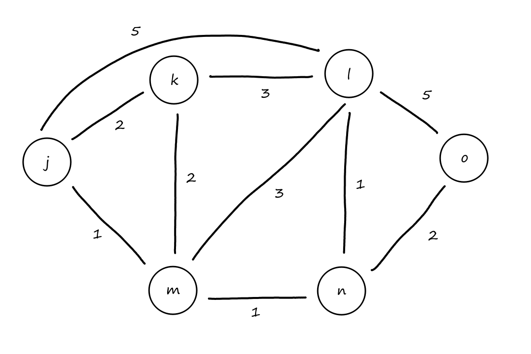
An edge has a numerical value representing its cost. In the context of networks, this value can be the physical length of the link, the speed of the link, or the monetary cost of using the link. The cost of the link is denoted by `c(x,y)`. If there is no edge that exists for nodes `x` and `y`, then `c(x,y)=oo`.
A path in a graph is a sequence of nodes and edges that can be traversed. The cost of a path is the sum of the cost of all the edges on that path.
A path is a sequence of `p` nodes `(x_1,x_2,...,x_p)` such that each of the pairs `(x_1,x_2),(x_2,x_3), ..., (x_(p-1),x_p)` are edges in the graph. The cost of a path is `c(x_1,x_2)+c(x_2,x_3)+...+c(x_(p-1),x_p)`.
For example, in the graph above, `(j,m,l,o)` is a path where the edges are `(j,m),(m,l),(l,o)`. The cost of this path is `c(j,m)+c(m,l)+c(l,o)=1+3+5=9`.
For any two nodes, there can be multiple paths between them. But at least one of them is the least costly. This path is the least-cost path. So the job of a routing algorithm is to find this least-cost path.
A routing algorithm can be centralized or decentralized. In a centralized routing algorithm, each node has complete knowledge about the whole network, so every node knows the cost of every edge. These algorithms are referred to as link-state (LS) algorithms, since they know the state of every link. In a decentralized algorithm, each node only has information about the cost of its neighbors, and they communicate with each other to gradually calculate the best path.
A routing algorithm can also be static or dynamic. In a static routing algorithm, routes change very slowly over time, often as a result of human intervention. In a dynamic routing algorithm, routes are dynamically updated in response to network topology or link cost changes.
A routing algorithm can also be load-sensitive or load-insensitive. In a load-sensitive algorithm, the link costs change to reflect the current level of congestion in the link. Load insensitive algorithms are the opposite.
The Link-State (LS) Routing Algorithm
In order for each node to have complete information about the network, they send link-state packets to all other nodes informing each other of its neighbors' costs. This is referred to as a link-state advertisement or a link-state broadcast. After this is done, each node will have an identical view of the network and can then run the LS algorithm.
One version of the LS algorithm is Dijkstra's algorithm. Dijkstra's algorithm is iterative. It keeps track of what the current least-cost path is so far, and, on every iteration, updates it as needed.
Yes, that Dijkstra.
Now, some notation. `D(v)` is the cost of the least-cost path from the source node to `v` as of the current iteration. `p(v)` is the previous node of `v` along the current least-cost path from the source to `v`. `N'` is the set of nodes where each node has a least-cost path calculated and determined.
This is the pseudocode for Dijkstra's algorithm. Let `u` be the source node.
Initialization:
`N' = {u}`
for all nodes `v`
if `v` is a neighbor of `u` then `D(v) = c(u,v)`
else `D(v)=oo`
Loop:
find `w` not in `N'` such that `D(w)` is a minimum
add `w` to `N'`
update `D(v)` for each neighbor `v` of `w` and not in `N'`:
`D(v)=min(D(v),D(w)+c(w,v))`
until `N'=N`
We'll use Dijkstra's algorithm on the graph above (copied and pasted below).
In the initialization step, we start at node `j` and calculate the cost to get to each node directly from `j`. Since `n` and `o` are directly unreachable from `j`, their cost on this iteration is `oo`.
| step | `N'` | `D(k),p(k)` | `D(l),p(l)` | `D(m),p(m)` | `D(n),p(n)` | `D(o),p(o)` |
|---|---|---|---|---|---|---|
| `0` | `j` | `2,j` | `5,j` | `1,j` | `oo` | `oo` |
In the first iteration, we look at the node with the current least cost (in this case, `m`) and go there. Then we calculate the cost to get to each of `m`'s neighbors from `m`. The cost to go to `k` from `m` is `3` (`1` for `jrarrm` and `2` for `mrarrk`), but it costs less to go to `k` from `j`, so we don't update `D(k),p(k)`. The cost to go to `l` from `m` is `4` (`1` for `jrarrm` and `3` for `mrarrl`), and it costs less than the current path to `l`, so we update `D(l),p(l)`. Node `n` is now reachable from `j`, so we update `D(n),p(n)`.
| step | `N'` | `D(k),p(k)` | `D(l),p(l)` | `D(m),p(m)` | `D(n),p(n)` | `D(o),p(o)` |
|---|---|---|---|---|---|---|
| `0` | `j` | `2,j` | `5,j` | `1,j` | `oo` | `oo` |
| `1` | `jm` | `2,j` | `4,m` | `2,m` | `oo` |
In the second iteration, we look at the node with the current least cost and go there. (There's a tie between `k` and `n`, so we'll just choose `n`.) Then we calculate the cost to get to each of `n`'s neighbors from `n`. The cost to go to `l` from `n` is `3` (`2` for `jrarrmrarrn` and `1` for `nrarrl`), and it costs less than the current path to `l`, so we update `D(l),p(l)`. Node `o` is now reachable from `j`, so we update `D(o),p(o)`.
| step | `N'` | `D(k),p(k)` | `D(l),p(l)` | `D(m),p(m)` | `D(n),p(n)` | `D(o),p(o)` |
|---|---|---|---|---|---|---|
| `0` | `j` | `2,j` | `5,j` | `1,j` | `oo` | `oo` |
| `1` | `jm` | `2,j` | `4,m` | `2,m` | `oo` | |
| `2` | `jmn` | `2,j` | `3,n` | `4,n` |
In the third iteration, we look at the node with the current least cost (in this case, `k`) and go there. It's important to note that for every iteration we do this, we have to pick the node that isn't in `N'` yet. The point of the algorithm is to visit every node so that we know what the least-cost path is from all nodes. (`N'` isn't the least-cost path; it's just the set of nodes that have been visited.) When looking at the neighbors, we also only look at the neighbors not in `N'` yet. So on this iteration, we only look at `l` (node `o` isn't a neighbor of `k`).
| step | `N'` | `D(k),p(k)` | `D(l),p(l)` | `D(m),p(m)` | `D(n),p(n)` | `D(o),p(o)` |
|---|---|---|---|---|---|---|
| `0` | `j` | `2,j` | `5,j` | `1,j` | `oo` | `oo` |
| `1` | `jm` | `2,j` | `4,m` | `2,m` | `oo` | |
| `2` | `jmn` | `2,j` | `3,n` | `4,n` | ||
| `3` | `jmnk` | `3,n` | `4,n` |
The table after finishing the algorithm looks like this:
| step | `N'` | `D(k),p(k)` | `D(l),p(l)` | `D(m),p(m)` | `D(n),p(n)` | `D(o),p(o)` |
|---|---|---|---|---|---|---|
| `0` | `j` | `2,j` | `5,j` | `1,j` | `oo` | `oo` |
| `1` | `jm` | `2,j` | `4,m` | `2,m` | `oo` | |
| `2` | `jmn` | `2,j` | `3,n` | `4,n` | ||
| `3` | `jmnk` | `3,n` | `4,n` | |||
| `4` | `jmnkl` | `4,n` | ||||
| `5` | `jmnklo` |
So now, for every node, we have the cost to get to that node, and that cost is the lowest cost possible. For example, it costs `3` to get to node `l`, and that path involves going there from `n`. It costs `2` to get to node `n`, and that path involves going there from `m`. It costs `1` to get to node `m`, and that path involves going there from `j`. Using this information, we can trim the graph so that only the least-cost paths are kept.
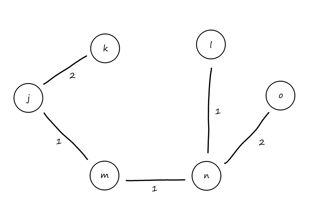
From this, we can create a forwarding table for all the routers to use:
| Destination | Link |
|---|---|
| `k` | `(j,k)` |
| `l` | `(j,m)` |
| `m` | `(j,m)` |
| `n` | `(j,m)` |
| `o` | `(j,m)` |
This algorithm is `O(n^2)`. In the first iteration, we process `n` nodes when calculating `D(v),p(v)`. In the second iteration, we process `n-1` nodes. In the (second-to-) last iteration we process `1` node. So the number of operations is `n+n-1+...+1=(n(n+1))/2`.
Using a heap to "find `w` not in `N'` such that `D(w)` is a minimum" can bring it down to `O(nlogn)`.
Suppose we have a network of four routers where the cost of each link is the measure of how much traffic is on that link. Let's say `x` has data of size `1` to send to `w`, `y` has data of size `elt1` to send to `w`, and `z` has data of size `1` to send to `w`. At the beginning, no data has been sent yet, so all the costs will be `0`.

After sending the data, the costs will now look like this:
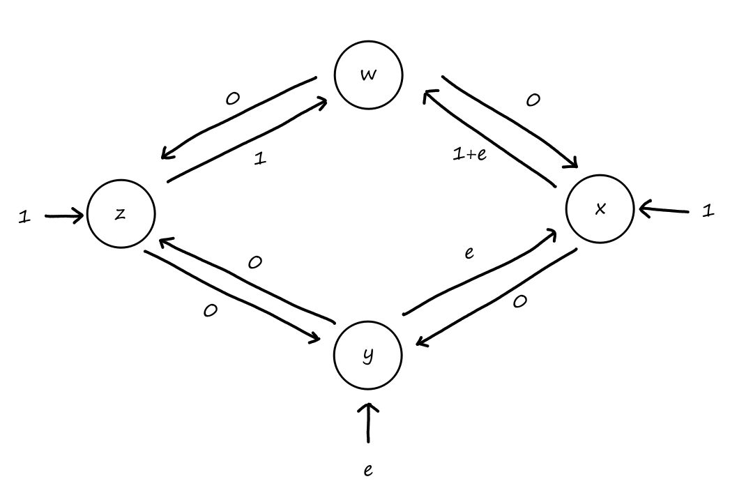
After running the LS algorithm, each router will take the clockwise path since that direction is the least-cost path:
After sending the data, the costs will now look like this:
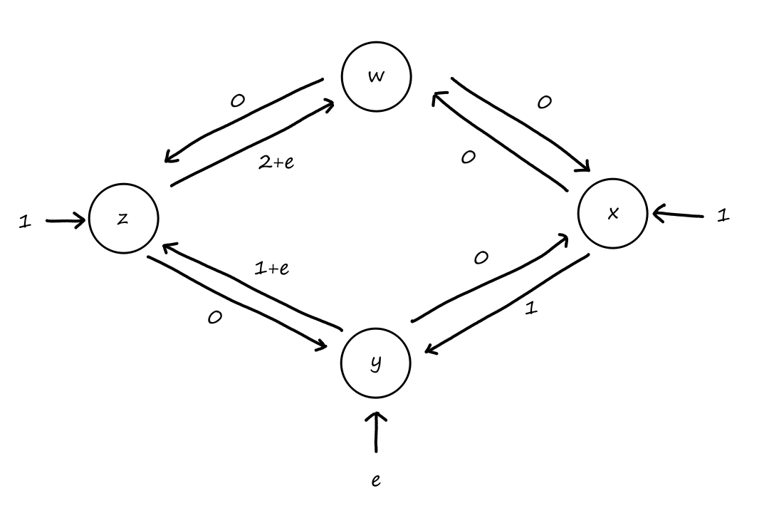
After running the LS algorithm, each router will take the counterclockwise path since that direction is now the least-cost path:
After sending the data, the costs will now look like this:
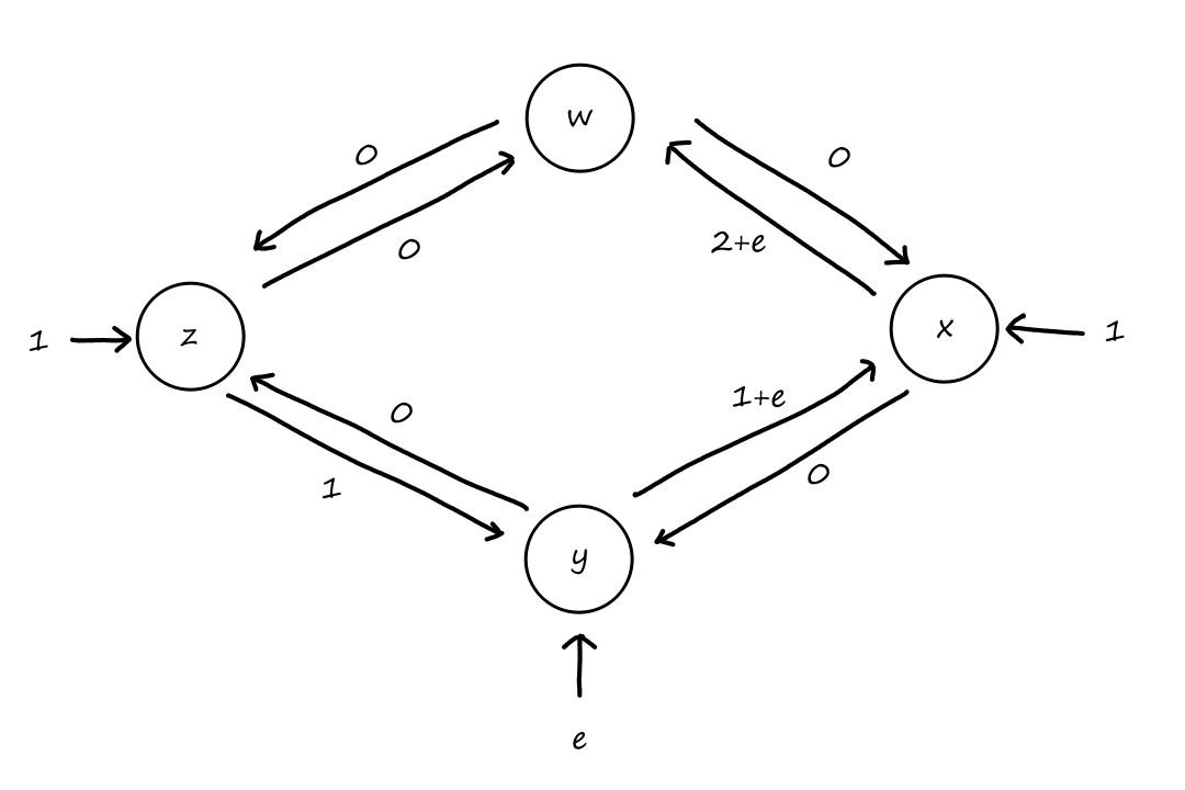
Notice that the routers will go back to sending the data clockwise again after running the LS algorithm. Earlier, we saw that if all the routers send the data clockwise, then they will send the data counterclockwise afterwards. After sending the data counterclockwise, they will send the data clockwise again. So the least-cost path will oscillate back and forth between clockwise and counterclockwise.
This is the result of using congestion as the measure of a link's cost. But we can't prevent congestion from being used as a metric since the whole point of routing is to avoid congested links. To prevent oscillation, the solution is to include randomness. So have the routers perform link-state advertisement at random times and have the routers run the LS algorithm at random times if the routers are using the traditional approach.
The Distance-Vector (DV) Routing Algorithm
One problem with the LS algorithm is that all the routers have to store the global information of the whole network. If there are a lot of routers in the network, then that's a lot of information for each router to store. So instead of having each router keep track of the whole network, each router can just keep track of its neighbors. Enter the distance-vector (DV) algorithm.
Let's say we wanted to deliver some package (as fast as possible ignoring cost) to some location that we can't get to ourselves. However, there are several delivery centers between us and the destination. Naturally, we would start by going to the nearest delivery center. There, we could tell them, "Deliver this to the destination, but use the best path possible." The delivery center will look at the next delivery center that's best for reaching the destination and send it there. Each delivery center will tell its next delivery center, "Deliver this to the destination, but use the best path possible" until the pacakge arrives at the destination. As long as the best path is used each time, the overall path will be the best.
Notice that we didn't have to know about all the delivery centers in the world; we only had to know the best delivery center for us. And similarly for each delivery center, each one only had to know about the delivery center that was best for it. (Of course, it's implied that for each delivery center, the next delivery center that is the best is one that can also reach the destination.)
The Bellman-Ford equation encompasses the idea above. Let `d_x(y)` be the cost of the least-cost path from node `x` to node `y`.
`d_x(y)=min_v{c(x,v)+d_v(y)}`
The Bellman-Ford equation says that for all neighbors `v` of `x`, look at their least-cost paths to `y` and the cost of going to that neighbor `v`.
For example, let's consider the least-cost path from `j` to `o`. Node `j` has three neighbors: `k`, `l`, and `m`.
- For `k`:
- the least-cost path to `o` has a cost of `5` (`krarrmrarrnrarro`)
- the cost to get to `k` is `2`
- For `l`:
- the least-cost path to `o` has a cost of `3` (`lrarrnrarro`)
- the cost to get to `l` is `5`
- For `m`:
- the least-cost path to `o` has a cost of `3` (`mrarrnrarro`)
- the cost to get to `m` is `1`
So `d_j(o)=min{2+5,5+3,1+3}=min{7,8,4}=4`.
Now for the actual DV algorithm. Each node begins with a list of costs from itself to every other node. Each node also keeps track of its neighbors' lists. From time to time, each node sends a copy of its own list to its neighbors. When a node receives a list from a neighbor, the node saves the neighbor's list and uses it to update its own list. If there were any changes, then that node will send its list to its neighbors. Initially, each node will start with a list of estimated costs, but eventually, the list will contain the actual costs.
Let `D_x(y)` be the estimated cost of the least-cost path from `x` to `y` for all `yinN`. Each node `x` begins with a distance vector `bbD_x(y)=[D_x(y):yinN]`. Each node also keeps track of its neighbors' distance vectors `bbD_v(y)=[D_v(y):yinN]` for neighbors `v` of `x`. Whenever a node `x` receives a distance vector from one of its neighbors, node `x` will update its own distance vector using the Bellman-Ford equation:
`D_x(y)=min_v{c(x,v)+D_v(y)}`
where `c(x,v)` is the cost of going to `v` from `x`
Initially, `D_x(y)` will be an estimated cost, but eventually, `D_x(y)` will converge to `d_x(y)`, which we denoted as the actual cost of the least-cost path from `x` to `y`.
This is the pseudocode for the Distance-Vector algorithm.
Initialization for each node `x`:
for all destinations `y` in `N`
`D_x(y)=c(x,y)`
for each neighbor `w`
`D_w(y)=?` for all destinations `y` in `N`
for each neighbor `w`
send distance vector `bbD_x(y)=[D_x(y):yinN]` to `w`
Loop over each node `x`:
wait until there is a link cost change to some neighbor `w` or until a distance vector is received from neighbor `w`
for each `y` in `N`
`D_x(y)=min_v{c(x,v)+D_v(y)}`
if `D_x(y)` changed for any destination `y`
send distance vector `bbD_x(y)=[D_x(y):yinN]` to all neighbors
We'll use the DV algorithm on a network of three nodes.
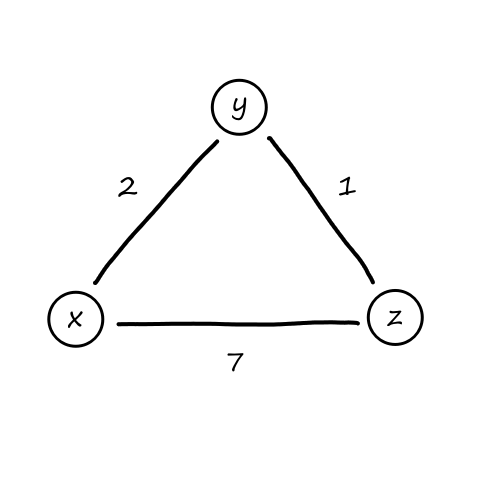
At the start, all three nodes will have their own initial routing tables (a row is a distance vector). Each node hasn't received the distance vector from their neighbors yet, so the values for each node's neighbors are `oo`.
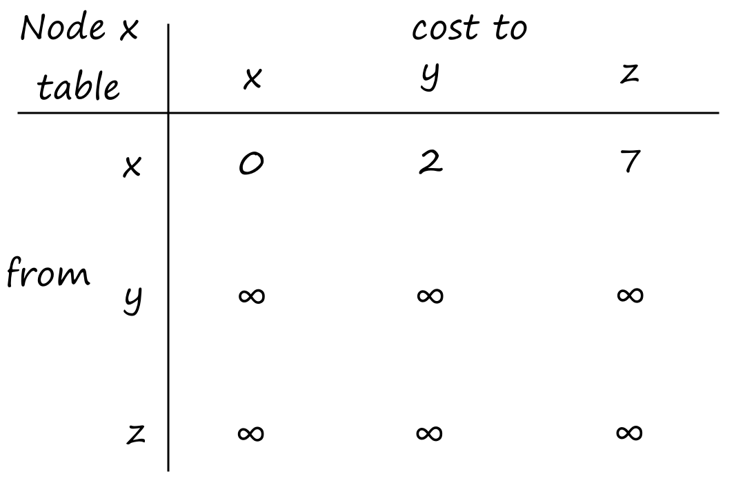

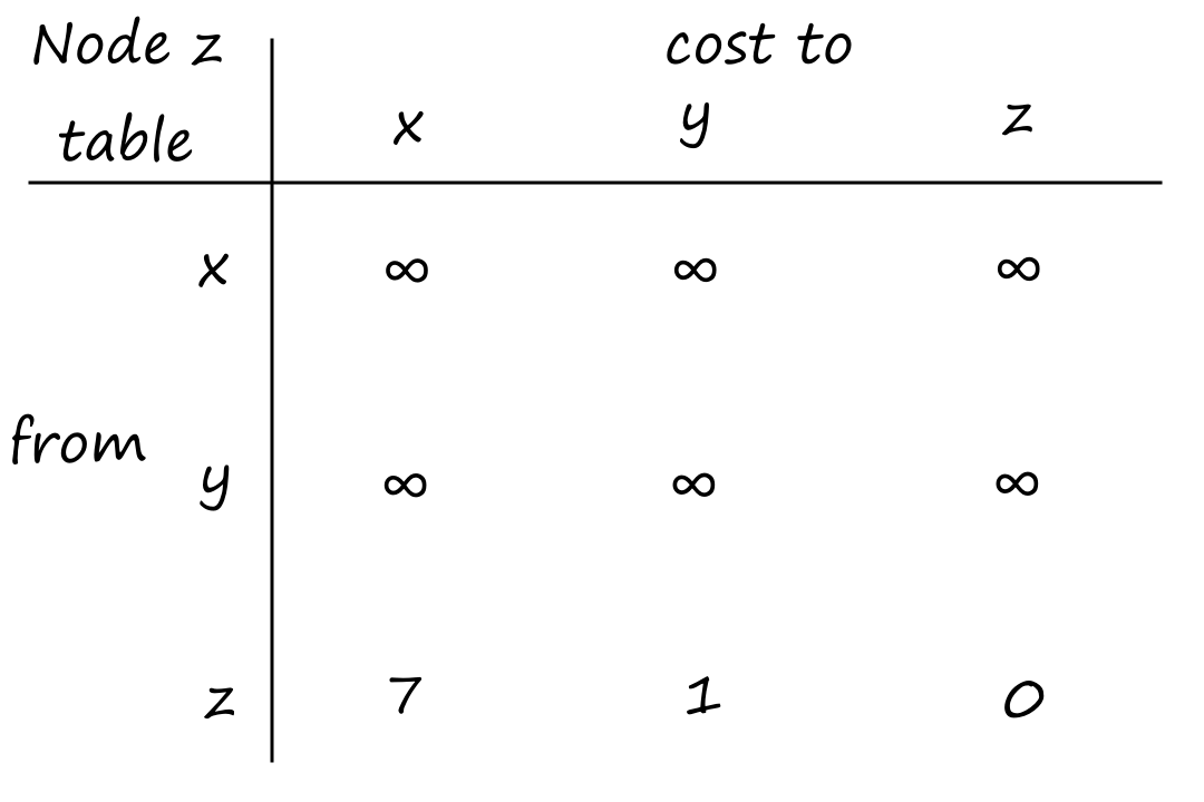
Now, each node will send their distance vector to their neighbors.


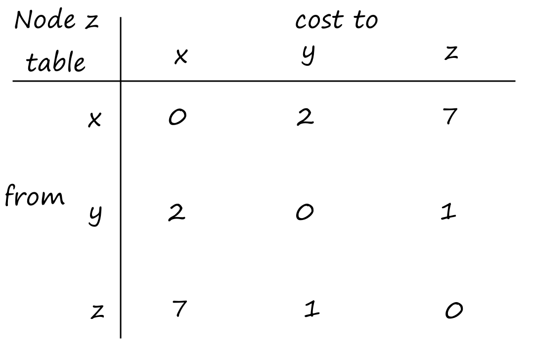
Upon receiving a distance vector from their neighbors, each node will update their own distance vectors. Let's start with `x`:
`D_x(y)=min{c(x,y)+D_y(y),c(x,z)+D_z(y)}=min{2+0,7+1}=min{2,8}=2`
`D_x(z)=min{c(x,y)+D_y(z),c(x,z)+D_z(z)}=min{2+1,7+0}=min{3,7}=3`
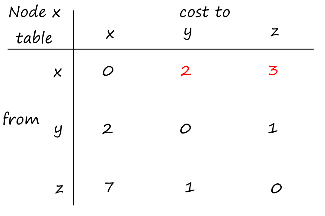
Since `x`'s distance vector changed, `x` will now send its updated distance vector to its neighbors. For `y`:
`D_y(x)=min{c(y,x)+D_x(x),c(y,z)+D_z(x)}=min{2+0,1+7}=min{2,8}=2`
`D_y(z)=min{c(y,x)+D_x(z),c(y,z)+D_z(z)}=min{2+7,1+0}=min{9,1}=1`
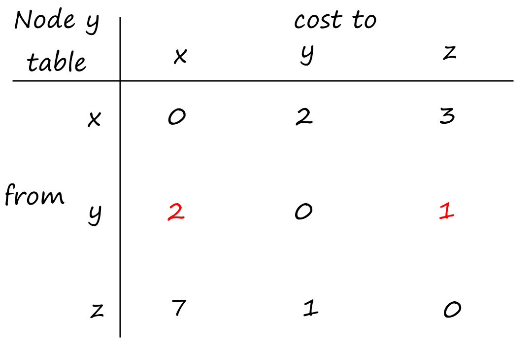
Notice that `y`'s distance vector did not change. So `y` will not send its distance vector to its neighbors.
We still have to calculate `z`'s distance vector as a result of `x` sending its distance vector to its neighbors:
`D_z(x)=min{c(z,x)+D_x(x),c(z,y)+D_y(x)}=min{7+0,1+2}=min{7,3}=3`
`D_z(y)=min{c(z,x)+D_x(y),c(z,y)+D_y(y)}=min{7+2,1+0}=min{9,1}=1`
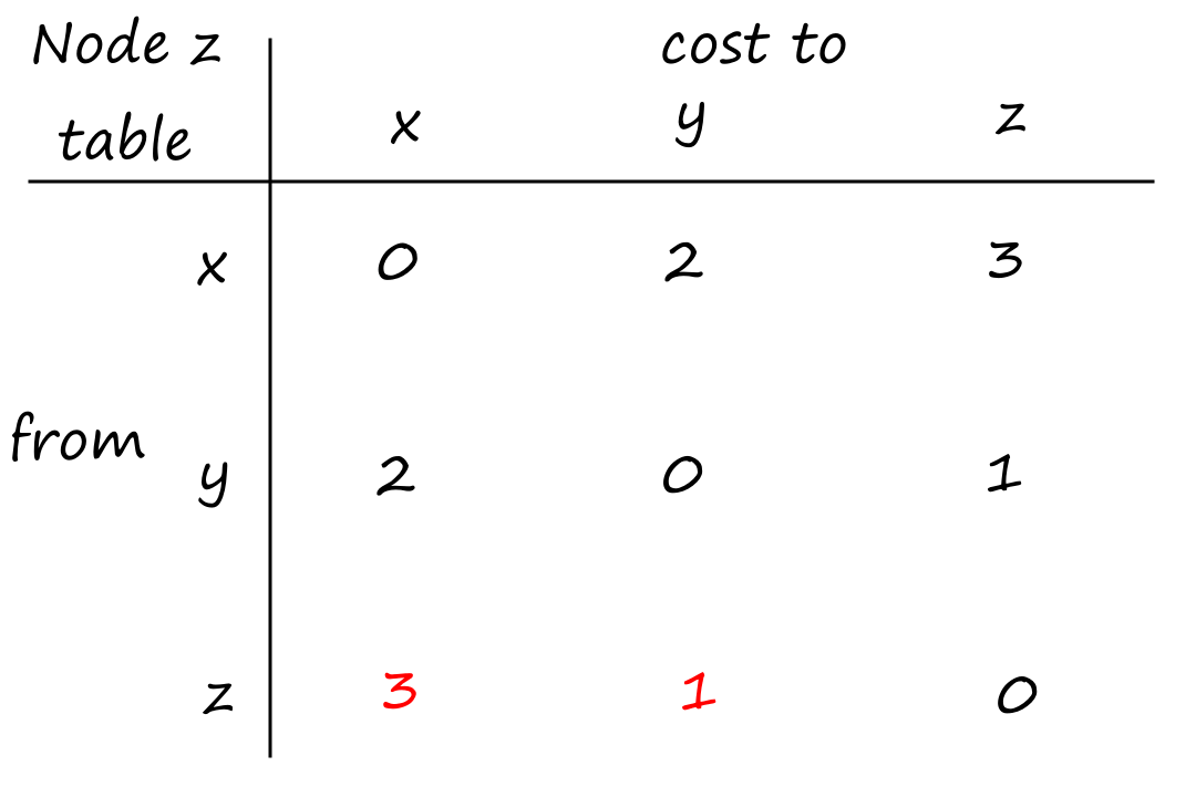
`z`'s distance vector changed, so `z` will send its updated distance vector to its neighbors. If we decide to continue with the math, we'll find that `x` and `y`'s distance vectors don't change from `z`'s updated distance vector. So the final routing table for all three nodes will look like the one above. At this point, since no nodes are sending distance vectors, all the nodes will just stay in a waiting state until there is a link cost change.
Even though we went through the example synchronously (starting with `x`, then updating `y` and `z`), the DV algorithm is asynchronous. So computing distance vectors and sending distance vectors can happen in any order at any time, depending on what happens to occur first. For example, instead of starting with `x`, we could've started with `y`.
The DV algorithm is also self-terminating. There is no explicit signal to stop; things just naturally stop when there is no updated information.
Link-Cost Changes and Link Failure
Let's look at the same three-node network but with different link costs this time.

Suppose the `x-y` link changes from `4` to `1` and that `y` detects this change first. `y`'s distance vector will be updated so that `D_y(x)=1` instead of `4`. Then, `y` will send its distance vector to its neighbors. When `z` gets `y`'s updated distance vector, `z` will update its own distance vector so that `D_z(x)=2`. (`x` will also update its own distance vector, but we'll only focus on `y` and `z` for this section.) Since `z`'s distance vector changed, `z` will send its distance vector to `y`, but `y`'s distance vector won't be changed, so everything will stop.
So things go normally if a link cost decreases. But what happens if the link cost increases? Let's say it increases from `4` to `60` instead.
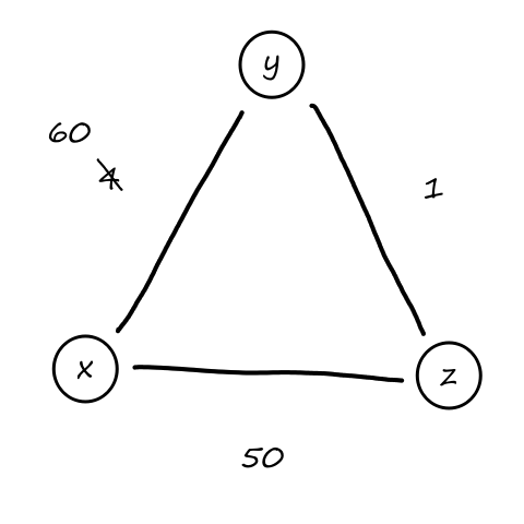
This is `y`'s table before `y` updates its distance vector.
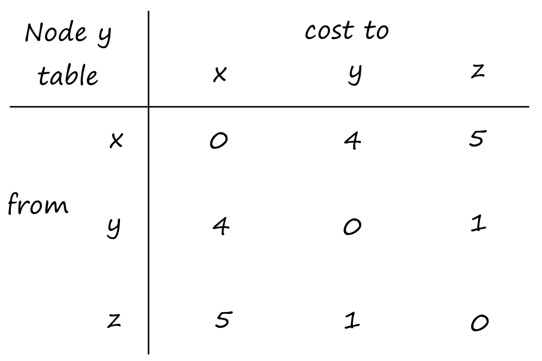
After detecting the link cost change, `y` will update its distance vector:
`D_y(x)=min{c(y,x)+D_x(x),c(y,z)+D_z(x)}=min{60+0,1+5}=6`
But this is clearly wrong since it's impossible to get from `y` to `x` with a cost of `6`. Of course, we can tell it's impossible since we have a global view of the network, but the nodes don't. This happened because `y` was using outdated information, namely `D_z(x)=5`; and this was outdated because `z` hadn't updated its distance vector yet.
At this point, there is also a routing loop. If `y` wants to send a packet to `x`, it will send it to `z` first since `y` thinks `z` can get to `x` with a cost of only `5`. But `z` can only get to `x` with a cost of `5` by going through `y`! (since `z` still believes `y` can get to `x` with a cost of `4`) So if there happens to be a packet to send at this time, then it will get bounced back and forth between `y` and `z`.
Since `y`'s distance vector changed, `y` will send its distance vector to `z`, which will update its distance vector by performing:
`D_z(x)=min{c(z,x)+D_x(x),c(z,y)+D_y(x)}=min{50+0,1+6}=min{50+7}=7`
These are the tables of `y` and `z` after `z` updates its distance vector:


Since `z`'s distance vector updated, `z` will send its distance vector to `y`, which will update its distance vector so that `D_y(x)=8`. Then `z` will update its distance vector so that `D_z(x)=9`. Then `y` will update its distance vector so that `D_y(x)=10`. And so on.
Eventually, `z` will perform the calculation:
`D_z(x)=min{c(z,x)+D_x(x),c(z,y)+D_y(x)}=min{50+0,1+50}=min{50+51}=50`
Finally, this will reflect the current state of the network: it is cheaper to go from `z` to `x` than it is to go from `z` to `y` to `x`.
However, it took several updates to get to that correct state. So if a link cost increases, it can potentially take a long time for the update to propagate among the nodes.
It would take even longer if the link cost had changed from `4` to `10,000` and the cost to go to `x` from `z` had been `9999`. Because of situations like this, this problem is referred to as the count-to-infinity problem.
Adding Poisoned Reverse
This can be avoided with a little trick called poisoned reverse. If the least-cost path from `z` to `x` is through `y`, then `z` will lie and tell `y` that `z` has no path to `x`, i.e., `D_z(x)=oo`. This way, `y` will not go through `z` to get to `x`.
Let's look at the example again but with poisoned reverse. The link cost changes from `4` to `60`, so `y` will update its distance vector. This time, `y` thinks that `D_z(x)=oo`, so `y` will calculate `D_y(x)` to be
`D_y(x)=min{c(y,x)+D_x(x),c(y,z)+D_z(x)}=min{60+0,1+oo}=60`
And `z` will update its `D_z(x)` to be
`D_z(x)=min{c(z,x)+D_x(x),c(z,y)+D_y(x)}=min{50+0,1+60}=50`
And in response, `y` will update its `D_y(x)` to be
`D_y(x)=min{c(y,x)+D_x(x),c(y,z)+D_z(x)}=min{60+0,1+50}=51`
which means that `y` is now going to `x` through `z`. And, since `y` is going to `x` through `z`, `y` will tell `z` that `y` has no path to `x`, i.e., `D_y(x)=oo`.
And just like that, all the nodes have the correct information about the current state of the network.
It's called poisoned reverse because the node is poisoning the reverse path so that the other node can't use it.
This poisoned reverse trick won't work for loops involving three or more nodes. The above example only had a two-node loop between `y` and `z`.
LS vs DV
Let `N` be the set of nodes (routers) and `E` be the set of edges (links).
| LS | DV | |
|---|---|---|
| Message Complexity | Since LS is global, each node needs to know about every other node and link. This means `O(|N||E|)` messages need to be sent on every run. | Since DV is decentralized, each node only needs to know about and exchange messages with its neighbors. |
| Speed of Convergence | LS takes `O(|N|^2)` time to complete. (For every node, we need to calculate the least-cost path to every other node.) | DV can converge slowly (from the count-to-infinity problem) and run into routing loops while converging. |
| Robustness (What if a router malfunctions?) | Since every node is computing their own forwarding table, route calculations are indpendent of each other across nodes. So if one node does a wrong calculation, only that node will have an incorrect forwarding table. | If one node spreads wrong information, that info will be propagated across the whole network. |
Neither algorithm is really that much better than the other. In the Internet, both of them are used.
Intra-AS Routing in the Internet: OSPF
So far, we've been assuming that all the routers are running the same routing algorithm. However, this isn't really practical because in the real world, there are billions of routers. All of them can't have enough memory to store this much information for LS. As for DV, running DV over this many routers would never converge.
Also recall that the Internet is a network of ISPs, which is a network of routers. An ISP can choose which algorithm it wants its routers to run. So each network of routers could potentially be running different algorithms anyway.
In fact, routers are organized into autonomous systems (ASs), where each AS is typically controlled by an ISP. All the routers in the same AS run the same routing algorithm and communicate within the AS. Regardless of whichever algorithm it is, the routing algorithm that is running in an AS is called an intra-autonomous system routing protocol.
Open Shortest Path First (OSPF)
OSPF is an intra-AS routing protocol that uses Dijkstra's algorithm, so each router will have a complete topological map of the network in the AS. Individual link costs are configured by network admins.
When talking about the LS algorithm, we looked at it as "given a set of costs, find the least-cost path". In practice, costs are assigned by network admins to influence where they want traffic to go. That is, the optimal paths are already known, and the network admin must find the right set of costs so that those optimal paths are prioritized.
For example, a link's cost can be inversely proportional to its capacity so that low-bandwidth links are not prioritized.
Link-state advertisements are sent to all the routers whenever there is a link change (e.g., cost change or status change) and every 30 minutes.
All messages exchanged between OSPF routers can be authenticated, which means that only trusted routers can talk to each other. This prevents attackers from forging OSPF messages and sending incorrect routing information.
OSPF messages are exchanged over the IP protocol, not TCP or UDP.
If there are multiple paths that have the same least cost, then they any/all of them can be used.
An OSPF system can be divided into areas. Each area runs its own LS algorithm and the routers broadcast to other routers in their area. Then there is a backbone area that is responsible for routing traffic to each of the different areas. And at the edge of each area, there is an area border router that transfers messages from the area to the backbone area.
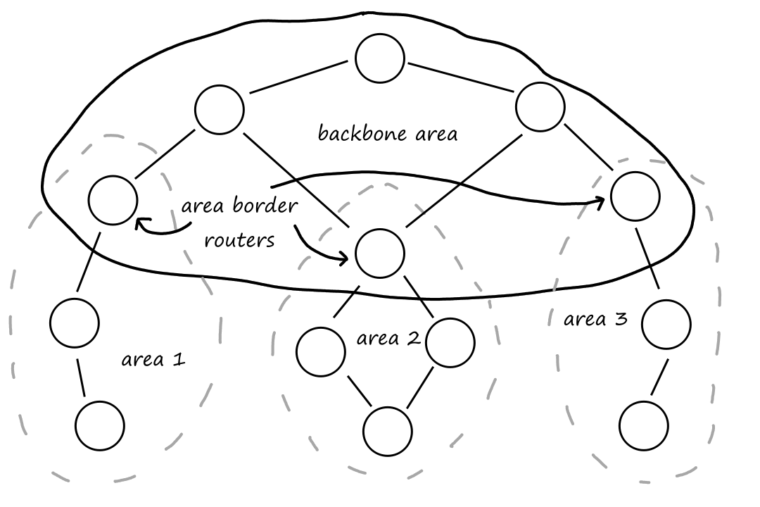
Routing Among the ISPs: BGP
An intra-AS routing protocol, like OSPF, routes packets from a source to a destination inside the AS. But to route a packet from one AS to another AS, an inter-autonomous system routing protocol is needed. And in order for the communication between ASs to work, they all need to be using the same inter-AS routing protocol. In fact, the inter-AS routing protocol that all ASs run is the Border Gateway Protocol, a.k.a. BGP.
The Role of BGP
A subnet is a smaller part of a larger network where all the IP addresses of the routers in the subnet start with the same prefix. BGP allows subnets to advertise their existence to all the routers in the Internet. And as mentioned earlier, BGP also determines the best route from one AS to another AS.
See the IPv4 Addressing section for more information about what a prefix is.
Advertising BGP Route Information
A router in an AS is either a gateway router or an internal router. A gateway router sits at the edge of an AS and connects to other routers in other ASs. An internal router only connects to hosts and routers in the AS.
Suppose we have a network with three autonomous systems: AS1, AS2, and AS3. Suppose AS3 includes a subnet with prefix x. We'll look at the details involved to make the routers in AS1 and AS2 aware of x.

When routers send messages to each other, they use semi-permanent TCP connections. A connection between routers is called a BGP connection. If the two routers communicating are in the same AS, then their connection is an internal BGP (iBGP) connection. If the two routers are in different ASs, then their connection is an external BGP (eBGP) connection.
So the steps for advertising the reachability information for x are:
- Gateway router 3a sends an eBGP message "AS3 x" to gateway router 2c.
- Gateway router 2c sends an iBGP message "AS3 x" to all the routers in AS2, including gateway router 2a.
- Gateway router 2a sends an eBGP message "AS2 AS3 x" to gateway router 1c.
- Gateway router 1c sends an iBGP message "AS2 AS3 x" to all the routers in AS1.
Determining the Best Routes
There can be more than one way to reach a prefix. Suppose, there's a connection from 1d to 3d.
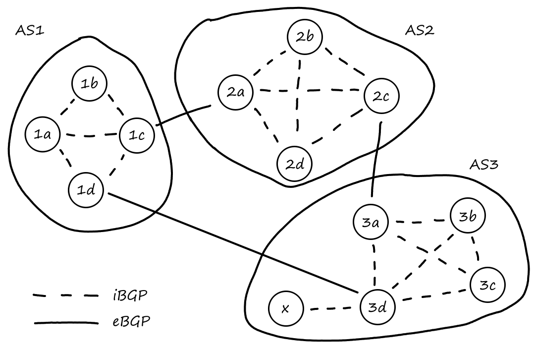
When a router sends a message advertising a prefix, it includes some BGP attributes. The prefix with its attributes is called a route.
The AS-PATH attribute is a list of ASs that the advertisement has passed through so far. When the message arrives at an AS, the AS adds itself to the AS-PATH list. But only if it isn't in the list yet to prevent loops.
There are two paths from AS1 to x:
- AS2 AS3 x
- AS3 x
The NEXT-HOP attribute is the IP address of the router at the beginning of the AS-PATH. For the route "AS2 AS3 x", the NEXT-HOP attribute is the IP address of router 2a. The NEXT-HOP attribute of the route "AS3 x" is the IP address of router 3d.
Hot Potato Routing 🥔
Hot potato routing tries to forward packets to other ASs as fast as possible. In this case, "fast" means "least cost".
Let's look at router 1b. This router has two paths to choose from: "AS2 AS3 x" and "AS3 x". Router 1b will use its intra-AS routing information to find the least-cost intra-AS path to 2a and and the least-cost intra-AS path to 3d and select the path with the smaller cost. We can define cost to be the number of links traversed for example. Then the cost of path "AS2 AS3 x" is `2` and the cost of path "AS3 x" is `3`, so 1b would choose path "AS2 AS3 x" and add router 2a to its forwarding table.
Route-Selection Algorithm
The actual process of choosing the best route is a little bit more complicated, but it does include hot potato routing.
- In addition to the AS-PATH and NEXT-HOP attributes, there is another attribute for a route's local preference. The local preference is decided by the AS's network admin. Routes with the highest local preference values are prioritized.
- If there are multiple routes with the same local preference values, then the route with the shortest AS-PATH is selected.
- If there are multiple routes with the same local preference values and the same AS-PATH length, then hot potato routing is used; so the route with the closest NEXT-HOP router is picked.
- If there are still multiple routes to choose from at this point, then BGP identifiers are used.
Let's look at router 1b again. We saw that it had two routes to choose from: one that went to AS2 and one that went to AS3. We also saw that under hot potato routing, the AS2 path is chosen. But under this new route-selection algorithm, rule 2 is applied before hot potato (rule 3). And rule 2 says to choose the route with the shortest AS PATH, which in this case is the route to AS3.
Routing Policy
For rule 1 of the route-selection algorithm, the local preference attribute is set by an AS routing policy. For example, a policy can prevent ASs from advertising a path to other ASs. ISPs may want to do this so that they don't have to forward traffic from customers that aren't subscribed to them.
For example, suppose we have six ASs where `W,X,Y` are access ISPs and `A,B,C` are provider networks. Suppose `A` advertises to `B` that there is a path to `W` through `A`. `B` can choose to advertise this path to `C`. Now `C` knows of a route to `W`, so if `Y` wants to communicate with `W`, then `C` can route through `B`.
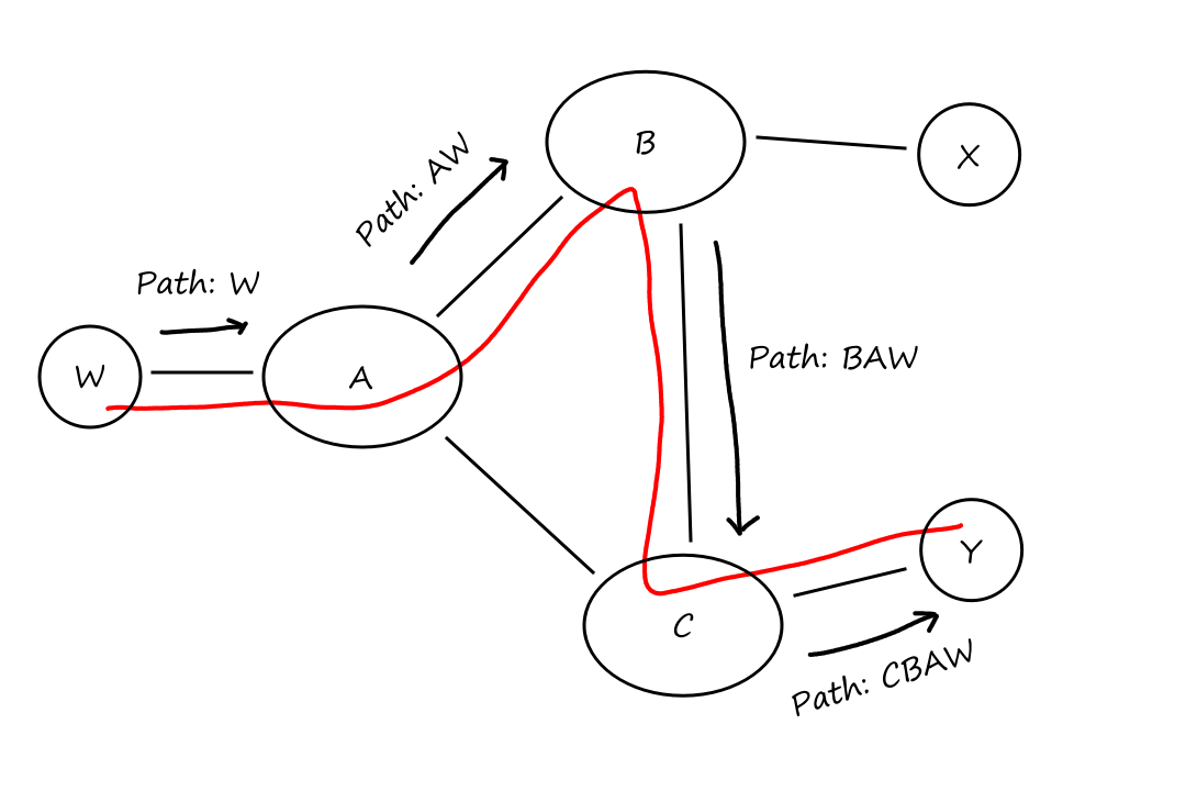
But now `B` can carry traffic between `Y` and `W`, both of which aren't customers of `B`. So it's in `B`'s interest to not advertise the path "BAW" to `C`.
IP-Anycast
IP-anycast is a service that allows multiple servers to share the same IP address. So when a request is sent to that IP address, any of the servers can pick up the request. This is helpful for CDNs and DNS since they both replicate their contents across multiple servers. BGP implements this IP-anycast service using the route-selection algorithm to select the "nearest" server.

Suppose a CDN company assigns the same IP address (212.21.21.21) to all of its servers. When routers receive advertisements for this IP address, they will think that there are multiple routes to the same location, when in fact they are in different locations. This way, the closest server can be used whenever content is requested from the CDN.
IP-anycast is actually not really used by CDNs because changes in routes can cause different packets of the same TCP connection to end up at different servers. IP-anycast is used more by DNS.
The SDN Control Plane
As we saw way, way back, SDN is the architecture where there is a controller that creates the forwarding tables and gives them to the switches (as opposed to the switches creating the tables themselves). There are four key characteristics:
- Flow-based forwarding: Packet forwarding rules are specified in a switch's flow table instead of being determined by the datagram's destination IP address.
- Separation of data plane and control plane: The data plane consists of the switches and the control plane consists of all the things that go into creating the flow table, including the controller.
- Programmable network: There are network-control applications that act as the "brains" of the SDN control plane. For example, a network-control application could run Dijkstra's algorithm to perform routing.
- Network control functions: There needs to be a way for the controller to communicate with the network-control applications because the controller maintains network state information and provides this to the applications.
SDN Controller
An SDN controller can be divided into three layers:
- Communication layer: The controller needs to communicate with the switches in the data plane (to send them their forwarding tables for example). The switches also need to communicate with the controller (to notify the controller that a new device has joined the network for example).
- Network-wide state management layer: In order to configure the flow tables, the controller needs to store all the information about the networks' hosts, links, switches, and other SDN devices, i.e., maintain the networks' states.
- Interface to the network-control application layer: This layer allows the controller to share its network state information with the network-control applications.
OpenFlow Protocol
The OpenFlow protocol is used by the controller to communicate with the switches (and vice versa). It uses TCP to transfer the messages.
There are four types of messages that a controller would send to a switch:
- set a switch's configuration parameters
- modify a switch's flow table
- ask a switch for information about its flow table
- send a packet out of a specific port at a switch
There are three types of messages that a switch would send to a controller:
- tell the controller that an entry in the flow table has been removed
- tell the controller that a port's status has changed (this is called a port-status message)
- send a packet to the controller (if there's nothing in the flow table for that packet)
Data and Control Plane Interaction: An Example
Suppose there is a link failure between one pair of switches.
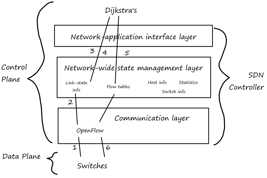
- One of the switches notifies the SDN controller that there is a link failure with an OpenFlow port-status message.
- The SDN controller receives the message and notifies the link-state manager.
- The link-state manager notifies the network-control application that there is a link-state change.
- The link-state routing application gets the updated link state from the link-state manager and computes new least-cost paths.
- The link-state routing application works with the flow table manager to determine which flow tables need to be updated.
- The flow table manager uses OpenFlow to update the flow table entries in the switches.
ICMP: The Internet Control Message Protocol
The Internet Control Message Protocol is used by hosts and routers to send network-layer information to each other. For example, a destination network could be unreachable. ICMP messages are carried in IP datagrams (the same way TCP/UDP segments are carried in IP datagrams).
ICMP messages have a type and a code. Some message types are shown here:
| ICMP Type | Code | Description |
|---|---|---|
| 0 | 0 | echo reply (to ping) |
| 3 | 0 | destination network unreachable |
| 3 | 1 | destination host unreachable |
| 3 | 2 | destination protocol unreachable |
| 3 | 3 | destination port unreachable |
| 3 | 6 | destination network unknown |
| 3 | 7 | destination host unknown |
| 4 | 0 | source quench (congestion control)* |
| 8 | 0 | echo request |
| 9 | 0 | router advertisement |
| 10 | 0 | router discovery |
| 11 | 0 | TTL expired |
| 12 | 0 | IP header bad |
*This is almost never used because TCP already has its own congestion control mechanism.
Traceroute
Traceroute is implemented using ICMP messages. It sends a bunch of IP datagrams to the destination, where each datagram contains a UDP segment with a port number that is unlikely to be open at the destination. The `n^(text(th))` datagram has a TTL of `n`, so when the `n^(th)` datagram arrives at the `n^(th)` router, the datagram will be expired*. In response, the router sends an ICMP warning message (type 11 code 0), which includes the name of the router and its IP address. When this message arrives at the source, Traceroute records the RTT.
*See the IPv4 Datagram Format section for more details about a datagram's TTL.
Since each subsequent datagram has a higher TTL, one of the datagrams will eventually reach the destination. When this happens, the destination will send a port unreachable ICMP message (type 3 code 3) back to the source. This is when Traceroute knows when to stop sending datagrams.
Network Management and SNMP
"Network management includes the deployment, integration, and coordination of the hardware, software, and human elements to monitor, test, poll, configure, analyze, evaluate, and control the network and element resources to meet the real-time, operational performance, and Quality of Service requirements at a reasonable cost." (Saydam & Magedanz 1996)
The Network Management Framework
A managed device is a device that connects to a network.
The managing server is an application that handles all the network managment information and commands to configure, monitor, and control the network's managed devices. This is managed by a network manager (a human).
Managed devices have configuration data (e.g., IP address), operational data (e.g., list of neighbors), and device statistics (e.g., number of dropped packets). The managing server also stores a copy of each device's data.
Managed devices also have a network management agent that communicates with the managing server.
The Simple Network Management Protocol (SNMP) and the Management Information Base (MIB)
A managed device's operational state data are stored as objects, which are combined into a Management Information Base (MIB). For example, an MIB could be a counter representing the number of IP datagrams discarded at a router due to errors in an IP datagram header. Related MIB objects are grouped into MIB modules.
SNMP is an application-layer protocol that allows for communication between the network management agent and the managing server. The most common usage is for the managing server to send a request to an agent to query or modify the data in a device's MIB. Another common usage is for an agent to send a trap message to the managing server to notify it of a situation that changed its MIB object values.
SNMP messsages are referred to as protocol data units (PDUs). They are usually carried in UDP datagrams.
| Type | Sender-receiver | Description |
|---|---|---|
| GetRequest | manager-to-agent | get value of one or more MIB object instances |
| GetNextRequest | manager-to-agent | get value of next MIB object instance in list/table |
| GetBulkRequest | manager-to-agent | get values in large block of data |
| InformRequest | manager-to-manager | inform remote managing entity of MIB values |
| SetRequest | manager-to-agent | set value of one or more MIB object instances |
| Response | agent-to-manager or manager-to-manager | generated in response to any of the above |
| Trap | agent-to-manager | inform manager of exceptional event |
Now to the data plane of the network layer!
What's Inside a Router?

The input port performs three functions. Once the data arrives at the router, the input port terminates the link at the physical-layer level, and the input port communicates with the link layer to do link-layer stuff. Then the input port performs a lookup in the forwarding table to determine the output port that the packet should be forwarded to.
A router's port is the physical input and output interface on the router. This is not the same "port" as the port number.
The switching fabric connects the router's input ports to its output ports.
The output port transmits packets received from the switching fabric to the router's outgoing link.
The routing processor runs control-plane functions. In traditional routers, the processor runs the routing protocols (OSPF and BGP) and creates the forwarding tables. In SDN routers, the processor gets the forwarding tables from the SDN controller and updates the entries in the input ports.
Because the data plane (input ports, switching fabric, output ports) has to work in nanoseconds, it is implemented in hardware. The control plane (routing processor) works in milliseconds or seconds, so it can be implemented in software.
Destination-Based Forwarding
The simplest type of forwarding is one based on a packet's destination address. Suppose a router has four links and that each link has a specified range of addresses it will take.
| Destination Address Range | Link Interface |
|---|---|
| 11001000 00010111 00010000 00000000 through 11001000 00010111 00010111 11111111 |
0 |
| 11001000 00010111 00011000 00000000 through 11001000 00010111 00011000 11111111 |
1 |
| 11001000 00010111 00011001 00000000 through 11001000 00010111 00011111 11111111 |
2 |
| anything that's not in the ranges above | 3 |
We can see that IP addresses that start with 11001000 00010111 00010 will go to link 0; addresses that start with 11001000 00010111 00011000 will go to link 1; addresses that start with 11001000 00010111 00011 will go to link 2. This leads to a simple forwarding table with only four rows:
| Prefix | Link Interface |
|---|---|
| 11001000 00010111 00010 | 0 |
| 11001000 00010111 00011000 | 1 |
| 11001000 00010111 00011 | 2 |
| anything that doesn't follow any of the patterns above | 3 |
So the router looks at the packet's destination address and matches it with a prefix in the table. But what happens if there is an address that matches more than one prefix? For example, 11001000 00010111 00011000 10101010 matches 1 and 2. If there are multiple prefixes that match, the router uses the longest prefix matching rule, which says to use the prefix that is the longest. So for the example, link 1 would be used.
Consider a network that uses 8-bit addresses. Suppose a router has the following forwarding table:
| Prefix | Link Interface |
|---|---|
| 00 | 0 |
| 010 | 1 |
| 011 | 2 |
| 10 | 2 |
| 11 | 3 |
For each of the four interfaces, what is the associated range of addresses and the number of addresses in the range?
Interface 0: 00000000 through 00111111 (64 addresses)
Interface 1: 01000000 through 01011111 (32 addresses)
Interface 2: 01100000 through 10111111 (96 addresses)
Interface 3: 11000000 through 11111111 (64 addresses)
Switching
A bus is a communication system that transfers data between components of a device. Only one packet can travel across the bus at a time.
There are several ways switching can be done. The first way is via memory. So the routing processor copies the packet into its memory, does the lookup in the forwarding table, and copies the packet to the output port's buffers.
From the input port to the routing processor and from the routing processor to the output port, the packet travels across the system bus twice. Because of this, if the routing processor can process a maximum of `B` packets per second, then the overall forwarding throughput is at most `B/2` (only one packet can travel across the bus at a time).
Switching can also be done via a bus. Instead of sending the packet to the routing processor, the input port transfers the packet directly to the output port over the bus. The input port puts a label on the packet indicating which output port the packet should go to. Then the bus transmits the packet to all the output ports, but only the output port that matches the label keeps the packet.
If multiple packets arrive at the router at the same time from different input ports, all but one have to wait since only one packet can travel across the bus at a time.
Switching can also be done via an interconnection network. Instead of having just one bus, there can be a bunch of buses that are interconnected. A crossbar switch is a type of interconnection network where there are `2N` buses for `N` input ports and `N` output ports.
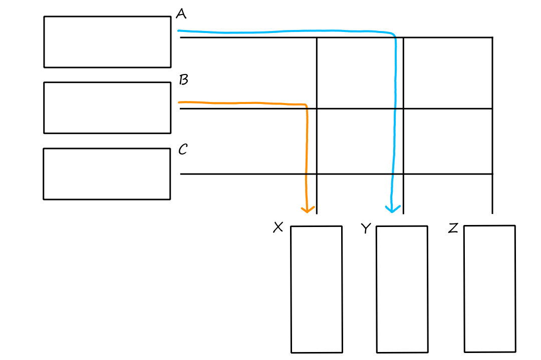
Here, there are three input ports `A,B,C`, three output ports `X,Y,Z`, three horizontal buses, and three vertical buses (for a total of six buses). This setup allows multiple packets to be forwarded at the same time because there are multiple buses. So a crossbar switch is non-blocking, as in it won't block other packets from being forwarded. Well, as long as they aren't going to the same output port, in which case, they would have to wait like before.
Port Queuing
Input ports and output ports have queues where packets wait to be switched from the input port or transmitted onto the link from the output port. When the queue gets full, packet loss can occur.
Input Queuing
At the input port, queuing will occur when the switching fabric is not fast enough. A crossbar switching fabric can help mitigate queuing since it allows multiple packets to be forwarded at once. But if multiple packets need to go to the same output port, then queuing will still happen. In fact, something called head-of-the-line (HOL) blocking can happen.
Suppose a packet in input port `A`'s buffer and a packet in input port `C`'s buffer need to go to output port `Z`. Let's say that the switch fabric gets the packet in `A` first. The pink packet in `C` has to wait for the purple packet to be switched first. But the red packet has to wait too, even though it's not going to `Z` and the bus from `C` to `X` is open.
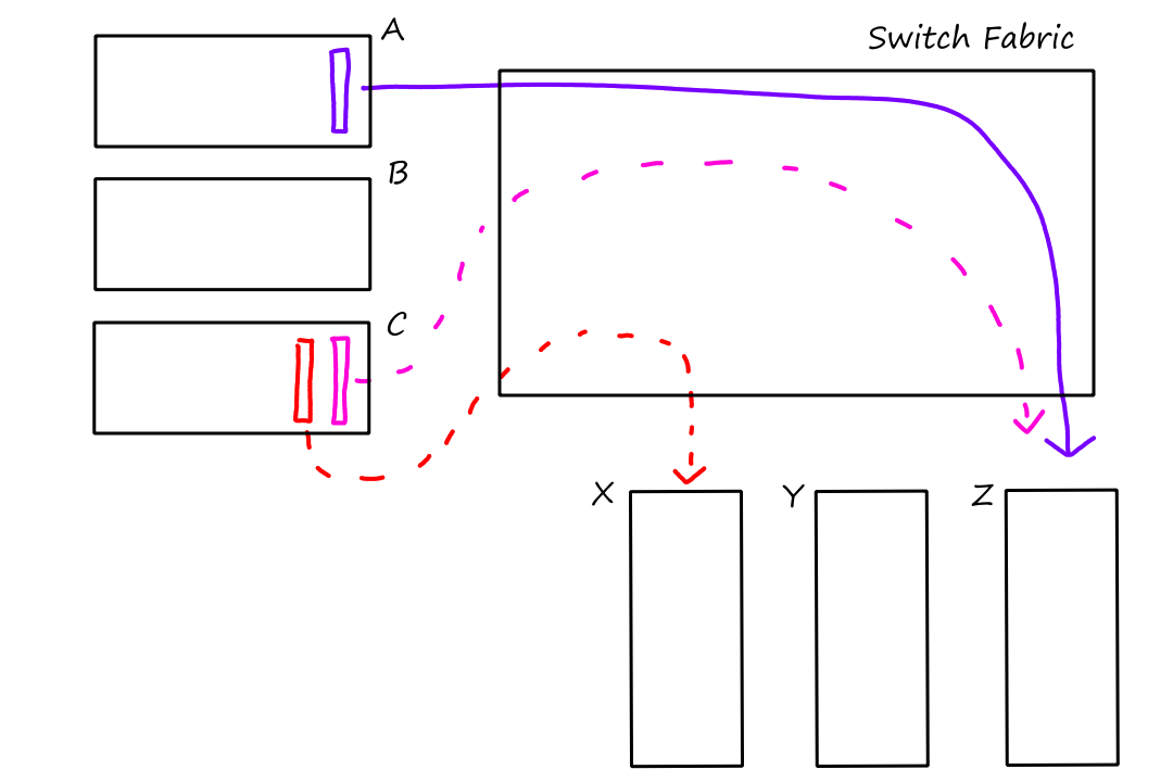
Output Queuing
At the output port, queuing will occur when the switching fabric is too fast (i.e., when the outgoing link's transmission rate is too slow). Output port queuing is more likely to happen than input port queuing since it is more likely that multiple packets from different input ports get forwarded to the same output port.
Packet Scheduling
When packets are sitting in the buffer, the port can decide which packets get transmitted first.
First-in-First-Out (FIFO)
This one is pretty self-explanatory. Packets get transmitted out of the queue in the same order that they came in the queue.
Priority Queuing
Packets can be classified by priority so that more important packets get put in a high-priority queue and less important packets get put in a low-priority queue. For example, packets for an Internet call can be considered more important than packets for an email*. If the router uses a non-preemptive priority queuing discipline, then higher-priority packets will not interrupt the transmission of lower-priority packets. That is, if a lower-priority packet is in the middle of being transmitted, the higher-priority packet will wait until it's done (even though it has a higher priority).
*These can be distinguished by looking at the source port number.
Round Robin
In round robin queuing, packets are organized into classes, but they all have equal priority. The router will alternate between each class and send one packet out from each class.
If the router uses a work-conserving queuing discipline, then it will move to the next class right away if there are no packets in that class (instead of waiting for a packet in that class to arrive).
Weighted Fair Queuing (WFQ)
This is similar to round robin, except that each class gets assigned a weight, indicating how many packets can be taken out when the router moves to that class. This is a generalized round robin, i.e., round robin is weighted fair queuing where all the weights are `1` (or the same number).
If each class `i` is assigned a weight `w_i`, then class `i` is guaranteed to receive bandwidth equal to `w_i/(sumw_j)`. For a link with transmission rate `R`, class `i` will have a throughput of `R*w_i/(sumw_j)`.
The Internet Protocol
There are two versions of IP currently in use: IPv4 and IPv6.
IPv4 Datagram Format
The following are included in an IPv4 datagram:
- Version number (`4` bits)
- Header length (`4` bits)
- used to determine where the data begins (since the header's length is variable)
- Type of service
- used to distinguish different types of datagrams (e.g., Internet call vs email)
- two of the bits are used for Explicit Congestion Notification
- Datagram length (`16` bits)
- Identifier, flags, offset
- used to rebuild an IP datagram that was broken up into smaller IP datagrams
- Time-to-live
- decremented by one each time the datagram is processed by a router
- if the TTL reaches `0`, the router must drop the datagram
- Protocol
- used to specify which transport-layer protocol is receiving this datagram
- Header checksum
- used to detect bit errors
- the checksum is computed the same way as we saw in the TCP section
- Source and destination IP addresses
- Options
- used to extend the IP header
- e.g., record IP addresses of routers it passed through, specify which routers to visit
- Data
+-+-+-+-+-+-+-+-+-+-+-+-+-+-+-+-+-+-+-+-+-+-+-+-+-+-+-+-+-+-+-+-+-+-+-+
| Version | Header length | Type of service | Datagram length (bytes) |
+-+-+-+-+-+-+-+-+-+-+-+-+-+-+-+-+-+-+-+-+-+-+-+-+-+-+-+-+-+-+-+-+-+-+-+
|       16-bit Identifier       | Flags | 13-bit Fragmentation offset |
+-+-+-+-+-+-+-+-+-+-+-+-+-+-+-+-+-+-+-+-+-+-+-+-+-+-+-+-+-+-+-+-+-+-+-+
| Time-to-live | Upper-layer protocol |        Header checksum        |
+-+-+-+-+-+-+-+-+-+-+-+-+-+-+-+-+-+-+-+-+-+-+-+-+-+-+-+-+-+-+-+-+-+-+-+
|                       32-bit Source IP address                      |
+-+-+-+-+-+-+-+-+-+-+-+-+-+-+-+-+-+-+-+-+-+-+-+-+-+-+-+-+-+-+-+-+-+-+-+
|                    32-bit Destination IP address                    |
+-+-+-+-+-+-+-+-+-+-+-+-+-+-+-+-+-+-+-+-+-+-+-+-+-+-+-+-+-+-+-+-+-+-+-+
|                          Options (if any)                           |
+-+-+-+-+-+-+-+-+-+-+-+-+-+-+-+-+-+-+-+-+-+-+-+-+-+-+-+-+-+-+-+-+-+-+-+
|                                 Data                                |
+-+-+-+-+-+-+-+-+-+-+-+-+-+-+-+-+-+-+-+-+-+-+-+-+-+-+-+-+-+-+-+-+-+-+-+
TCP/UDP can theoretically run over a different network-layer protocol besides IP. Likewise, IP can carry data to a different transport-layer protocol besides TCP/UDP.
With the TCP/IP combo, error checking is done at both layers, which may seem repetitive*. But if another combination is used, then there's no guarantee that error checking will be performed at all. So it's nice to have at least one protocol in each layer that can perform error checking.
*In IP's error checking, only the header is checksummed. While in TCP's error checking, the whole segment is checksummed. So the error-checking process isn't exactly repeated in both layers.
If there are no options, then an IP datagram's header is `20` bytes. If the datagram is carrying a TCP segment, then there will be a total of `40` bytes of header along with the application message.
IPv4 Addressing
An interface is the boundary between a host and the physical link into the network. Technically, an IP address is an identifier for an interface, not a device.
If we think of a router as a laptop, then an interface can be thought of as a USB port. A laptop with three USB ports has three interfaces and each interface gets its own IP address.
Actually, a laptop (sometimes) has two ways of connecting to the Internet: WiFi and Ethernet. This is why the IP address when using WiFi is different than the IP address using Ethernet; there are two interfaces.
An IP address is `32` bits (`4` bytes) long. They are represented in dotted-decimal notation, so each byte is represented as a decimal number and separated by a dot. For example, 193.32.216.9 is the dotted-decimal form of 11000001 00100000 11011000 00001001.
There are `2^32` (~`4` billion) possible IP addresses.
IP addresses aren't randomly generated; a part of it is determined by what subnet the interface is connected to.
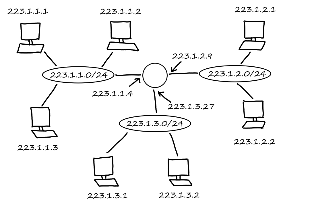
In this setup, there is one router with three interfaces connecting seven hosts. The three left hosts are connected to one subnet; the two right hosts are connected to another subnet; the bottom two hosts are connected to another subnet.
The left hosts and the interface they're connected to all have IP addresses that look like 223.1.1.*, i.e., their IP addresses all have the same leftmost `24` bits. One IP address is assigned to that subnet: 223.1.1.0/24. The /24 is a subnet mask indicating the fact that the leftmost `24` bits define the subnet address.
So why does everything in a subnet have similar looking addresses? It's because of the Internet's address assignment strategy, which is called Classless Interdomain Routing (CIDR). CIDR divides an IP address into two parts so that it looks like a.b.c.d/x where x indicates the number of bits in the first part.
An organization is usually given a block of contiguous addresses, i.e., a bunch of addresses that start with the same bits. This set of shared bits is the prefix (a.k.a. network portion) of the address, and x indicates how many bits make up the prefix, i.e., how long the prefix is. The remaining bits (a.k.a. the host part) are used as identifiers for the devices in the organization. In the example above for the left subnet, the prefix is 223.1.1 and the three hosts are identified by the 1, 2, and 3 at the end.
Having subnets reduces the amount of memory needed since the forwarding tables only need to store the prefix instead of the IP addresses of all the routers in the subnet.
Before CIDR, classful addressing was used, which only allowed the prefix to be `8`, `16`, or `24` bits long. This was because subnets with `8`-, `16`-, and `24`-bit subnet addresses were called class A, B, and C networks, respectively. But fixing the length of the prefix became an issue, especially for small-to-medium-sized organizations.
A class C subnet could only support `254` hosts, which was too small.
Since `24` bits are used for the prefix, there are `8` bits left to assign to hosts. So there are `2^8=256` assignable addresses. Actually, `254` since `2` of the addresses are reserved for special use.
A class B subnet could support `65,634` hosts, which was too large. If an organization only had `2000` hosts, then more than `63,000` addresses would be unused. Furthermore, they couldn't be used by any other organization.
Since `16` bits are used for the prefix, there are `16` bits left to assign to hosts. So there are `2^16=65,536` assignable addresses. And again, `2` of the addresses are reserved for special use, so `65,634`.
Another type of IP address is the broadcast address: 255.255.255.255. When a host sends a datagram with this destination address, the message is sent to all hosts on the same subnet.
The broadcast address (all `1`s) and the address consisting of all `0`s are the two addresses reserved for special use.
Obtaining a Block of Addresses
So how do these addresses get assigned? An ISP could be given an address block, let's say 200.23.16.0/20. Then the ISP could divide its block into smaller equal-sized address blocks for the organizations that the ISP supports. Let's say the ISP divides it into `8` address blocks. (The subnet part is underlined.)
| ISP's block | 200.23.16.0/20 | 11001000 00010111 00010000 00000000 |
| Organization 1 | 200.23.16.0/23 | 11001000 00010111 00010000 00000000 |
| Organization 2 | 200.23.18.0/23 | 11001000 00010111 00010010 00000000 |
| Organization 3 | 200.23.20.0/23 | 11001000 00010111 00010100 00000000 | `vdots` | `vdots` | `vdots` |
| Organization 8 | 200.23.30.0/23 | 11001000 00010111 00011110 00000000 |
Getting them from an ISP is not the only way to get a block addresses. (There has to be a way for the ISP itself to get a block of addresses in the first place!) The Internet Corporation for Assigned Names and Numbers (ICANN) is the global authority for managing and allocating IP addresses.
Consider a router that interconnects three subnets. Suppose all of the interfaces in each of these three subnets are required to have the prefix 223.1.17/24. Also suppose that Subnet 1 is required to support `120` interfaces, Subnet 2 is to support `60` interfaces, and Subnet 3 is to support `60` interfaces. What are three network addresses (of the form a.b.c.d/x) for each subnet that satisfy these constraints?
First of all, 223.1.17 in binary is 11011111 00000001 00010001 00000000. The subnet mask is /24, so the prefix for all the subnets is the underlined part of 11011111 00000001 00010001 00000000.
This means that only the last `8` bits are for address assignment. Using all `8` bits means that there are `2^8-2=254` addresses that can be assigned. But Subnet 1 is required to support only `120` interfaces, so we don't need to use all `8` bits. Using `7` bits means that there are `2^7-2=126` assignable addresses, so that's good enough for Subnet 1. If we only need `7` bits, then the remaining bit must be part of the prefix for Subnet 1.
So a network address for Subnet 1 is 11011111 00000001 00010001 00000000, a.k.a. 223.1.17.0/25.
Using `6` bits means that there are `2^6-2=62` assignable addresses, which is good enough for Subnet 2 and Subnet 3. And the remaining two bits must be part of the prefix for Subnet 2 and Subnet 3, which means their subnet masks will be /26.
The `128` addresses* from 223.1.17.0 to 223.1.17.127 are reserved for Subnet 1. So the `64` addresses starting from 223.1.17.128 can be used for Subnet 2. This network address is 223.1.17.128/26.
The `64` addresses from 223.1.17.128 to 223.1.17.191 are reserved for Subnet 2. So the `64` addresses starting from 223.1.17.192 can be used for Subnet 3. This network address is 223.1.17.192/26.
*There are `128` addresses, but only `126` are assignable. The address where the host part is all 0s and the address where the host is all 1s (the broadcast address) are reserved.
Consider a router and three attached subnets A, B, and C. Subnet A can support `24` hosts; Subnet B can support `53` hosts; and Subnet C can support `238` hosts. The subnets share the `23` high-order bits of the address space: 172.19.106.0/23.
How many hosts can there be in this address space?
The subnet mask is /23, so the last `9` bits can be used for hosts. There are `2^9=512` possible addresses. However, the first and the last (broadcast) address can't be assigned to hosts, so there are `510` addresses available for hosts.
Assign subnet addresses to each of the subnets (A, B, and C) so that the amount of address space assigned is minimal, and at the same time leaving the largest possible contiguous address space available for assignment if a new subnet were to be added. (This requirement just means start with the subnet that has the highest number of hosts and continue in decreasing order.)
Hint: it might help to first find the range of possible addresses to help visualize things.
(The relevant parts of) 172.19.106.0 in binary is 172.19.01101010.00000000. Since the last `9` bits can be used for hosts, the range of possible addresses is
172.19.01101010.00000000 - 172.19.01101011.11111111
(`2^9=512` possible addresses)
Since C has the highest number of hosts, we'll start with C. We need `2^8=256` addresses to support C's `238` hosts. This means the range of addresses for C is
172.19.106.0 - 172.19.106.255
So the subnet address of C is 172.19.106.0/24.
B has the next highest number of hosts. We need `2^6=64` addresses to support B's `53` hosts. This means the range of addresses for B is
172.19.107.0 - 172.19.107.63
So the subnet address of B is 172.19.107.0/26.
Lastly, A. We need `2^5=32` addresses to support A's `24` hosts. This means the range of addresses for A is
172.19.107.64 - 172.19.107.95
So the subnet address of A is 172.19.107.64/27.
What is the broadcast address of subnet A?
The broadcast address is the last address in the range, which for A is 172.19.107.95.
What is the starting address of subnet A? ("Starting" means "usable by a host".)
Since the first address (172.19.107.64) can't be used, the starting address is 172.19.107.65.
What is the ending address of subnet A? ("Ending" means "usable by a host".)
Since the broadcast address (172.19.107.95) can't be used, the ending address is 172.19.107.94.
Obtaining a Host Address
When an organization gets a block of addresses, it can manually assign addresses to the hosts and routers in the organization (meaning that a system admin would go to each device and configure the settings). But it's better to have that automated so that new hosts joining the network can automatically be assigned an IP address. This is done by using the Dynamic Host Configuration Protocol (DHCP). DHCP can be configured so that a host gets the same IP address each time it connects to the network, or it can be given a temporary IP address that will be different each time.
Because everything is done automatically, DHCP is called a plug-and-play or zeroconf (zero-configuration) protocol.
DHCP is a client-server protocol where the client is a host that wants to connect to the network. Either a subnet has a DHCP server or the subnet is connected to a router that knows a DHCP server.
There are four steps involved for getting an IP address using the DHCP protocol:
- The client tries to find a DHCP server using a DHCP discover message.
- Each DHCP server that gets the message responds with a DHCP offer message. The offer message contains the proposed IP address, the network mask, and an IP address lease time, which is the amount of time that the address is valid for.
- The client chooses an offer message and responds with a DHCP request message.
- The server responds with a DHCP ACK message.
When a client is trying to join a network, it won't know the IP address of any DHCP servers (since it's not connected to the network). So what destination address does the client use to send the discover message? It uses 255.255.255.255 to reach all the devices in the network.
Likewise, when a DHCP server sends an offer message, it also has to use 255.255.255.255 because the client hasn't been assigned an IP address yet.
The IP address lease time is typically hours or days, but DHCP has a renew mechanism that allows a client to renew its lease on an IP address.
Network Address Translation (NAT)
Earlier we saw that ISPs divide their address blocks into smaller blocks and distributes them to their customers. But what if some customers have so many devices that need to connect to the Internet? The ISP has already divided its address block and distributed them, so it's not like they can just increase the range of addresses.
Instead of giving a range of addresses to customers, ISPs can give only one address. Then the organization's network can be set up using fake IP addresses.
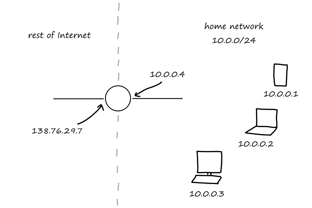
For example, suppose our ISP gave us an IP address of 138.76.29.7. Then when our home network is set up, a fake subnet of 10.0.0/24 is created. So the phone, laptop, and computer are given fake IP addresses. If those devices want to communicate with each other, then they can identify each other using the fake addresses. But if any devices outside of the home network need to communicate with the devices in the home network (and vice versa), then those fake IP addresses won't work because they're not real. So the fake address (e.g., 10.0.0.1) needs to be translated into the real address (138.76.29.7). This is network address translation (NAT).
The NAT-enabled router looks like a single device to the rest of the Internet. So all traffic coming out of the home network looks like it's coming from one device. This means that, in our example, the source IP address of all datagrams sent by the phone, laptop, and computer is 138.76.29.7.
This also means that all traffic going to the home network (regardless of whoever the receiver is) needs to go to one destination IP address: 138.76.29.7. But then how does the router know which device it's supposed to go to?
When the host sends a datagram, it puts an arbitrary port number in the source port field. Then the NAT router generates a new source port number for that datagram and puts that mapping into its NAT translation table. So the NAT translation table is used to know which device to send the data to.
| NAT Translation Table | |
|---|---|
| 138.76.29.7, 5001 | 10.0.0.2, 3345 |
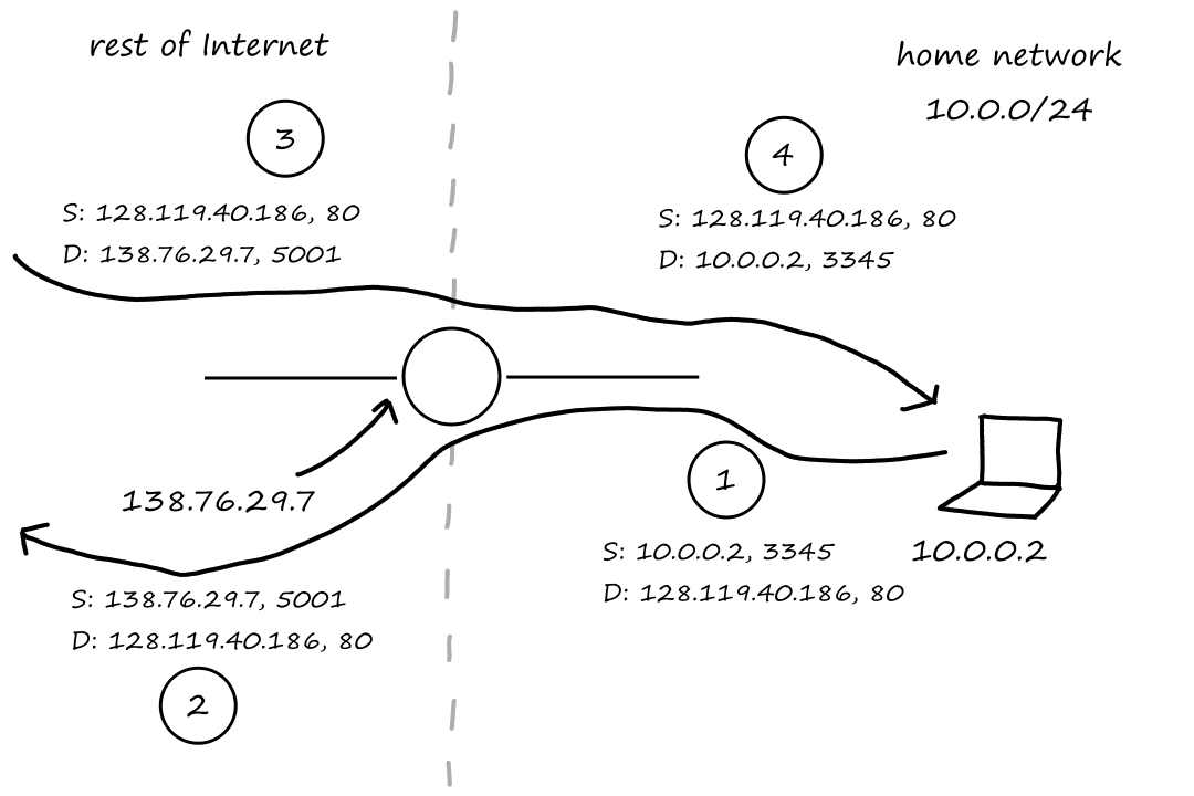
For example, let's say the laptop requests a Web page from 128.119.40.186.
- The laptop gives itself a port number of 3345 and sends a datagram to the router with source IP address 10.0.0.2 and source port number 3345.
- The NAT router generates a new source port number 5001, translates the IP address to the real one, and sends the datagram to the Web server at 128.119.40.186.
- The Web server sends the Web page to the NAT router (at the real IP address).
- The NAT router looks at its translation table to find the correct destination.
Since the port number field is `16` bits long, the NAT protocol can support up to `2^16=65,536` devices with just one IP address.
Benefits of NAT:
- range of addresses not needed from ISP
- can change addresses of devices in local network without notifying outside world
- can change ISP without changing addresses of devices in local network
- devices inside local network are not explicitly addressable (they're not visible to potential attackers)
Arguments against NAT:
- port numbers are meant to address processes, not hosts
- routers should only process network-layer things (like IP address), but modifying the port number is a transport-layer thing
- we should be using IPv6 instead of IPv4 (to handle the address shortage)
- violates the principle that hosts should be able to communicate with each other without any intermediaries
- this makes it harder for some applications, like P2P applications, to work properly
IPv6
Using `32` bits for an IP address means that there are only `2^32=4,294,967,296` addresses available. With the growing number of devices, this number is really small. And in fact, the last remaining pool of unassigned IPv4 addresses was allocated in February 2011.
So what about IPv5? There was a protocol called ST-2 that was supposed to become IPv5, but ST-2 was dropped.
IPv6 Datagram Format
The main improvements from IPv4 are that `128` bits are used for IP addresses and that the header is fixed to `40` bytes. The concept of a flow was also introduced where a bunch of packets may be treated as a flow of packets.
+-+-+-+-+-+-+-+-+-+-+-+-+-+-+-+-+-+-+-+-+-+-+-+-+-+-+-+-+-+-+-+-+
|Version| Traffic class |           Flow label                  |
+-+-+-+-+-+-+-+-+-+-+-+-+-+-+-+-+-+-+-+-+-+-+-+-+-+-+-+-+-+-+-+-+
|         Payload length        |  Next header  |   Hop limit   |
+-+-+-+-+-+-+-+-+-+-+-+-+-+-+-+-+-+-+-+-+-+-+-+-+-+-+-+-+-+-+-+-+
|                                                               |
+                   Source address (128 bits)                   +
|                                                               |
+-+-+-+-+-+-+-+-+-+-+-+-+-+-+-+-+-+-+-+-+-+-+-+-+-+-+-+-+-+-+-+-+
|                                                               |
+                 Destination address (128 bits)                +
|                                                               |
+-+-+-+-+-+-+-+-+-+-+-+-+-+-+-+-+-+-+-+-+-+-+-+-+-+-+-+-+-+-+-+-+
|                                                               |
+                             Data                              +
|                                                               |
+-+-+-+-+-+-+-+-+-+-+-+-+-+-+-+-+-+-+-+-+-+-+-+-+-+-+-+-+-+-+-+-+
The following are included in an IPv6 datagram:
- Version number (`4` bits)
- Traffic class (`8` bits)
- used to assign priority
- Flow label (`20` bits)
- Payload length (`16` bits)
- Next header
- used to specify which transport-layer protocol is receiving this datagram
- (same as protocol field in IPv4)
- Hop limit
- decremented by one each time the datagram is processed by a router
- (same as TTL field in IPv4)
- Source and destination IP addresses
- Data
In IPv4, there were three fields used for datagram fragmentation and reassembly. In IPv6, routers are not allowed to break up datagrams into smaller pieces. Instead, if the datagram is too large, the router drops the datagram and sends an ICMP error message ("Packet Too Big") to the sender.
The header checksum was also removed, because error checking was already (assumed to be) performed in the transport layer and link layer.
The options field in IPv4 is not explicitly defined in IPv6. Instead, it can be included in the next header field if needed.
Transitioning from IPv4 to IPv6
While IPv6-capable devices can be introduced easily into the existing Internet (i.e., it's backward-compatible so that it can handle IPv4 datagrams), the existing IPv4 devices aren't capable of handling IPv6 datagrams.
The transition has been handled by a concept called tunneling. Suppose an IPv6 router wants to send an IPv6 datagram to another IPv6 router, but there is an IPv4 router in between them. The IPv6 router creates an IPv4 datagram and puts the whole IPv6 datagram in the data field of the IPv4 datagram. It also puts (the protocol number for) IPv6 in the protocol field. So when the IPv4 router receives the datagram, it is unaware that the datagram actually contains an IPv6 datagram; it treats it just like any other datagram and sends it to the next destination. When the other IPv6 router gets the IPv4 datagram from the IPv4 router, it looks at the protocol field to know that the datagram actualy contains an IPv6 datagram.
It's called tunneling because the IPv4 router(s) in between the IPv6 routers are seen as a tunnel.
Generalized Forwarding and SDN
Recall that forwarding is the process of moving a packet from a router's input port to the router's output port by looking at the router's forwarding table. This is a "match-plus-action" pattern where looking at the forwarding table is a "match" and sending the packet to the switching fabric is an "action".
For traditional routers (as opposed to SDN routers), the forwarding table consisted of destination IP addresses. So an IP address would be mapped to an output link (see the Destination-Based Forwarding section).
But for SDN routers, their tables contain forwarding rules that are determined by multiple header fields. The forwarding table is called a flow table.
The flow table has three columns. The first column is the set of header field values that the packet switch uses for lookup. A packet "matches" a flow table entry if its headers are found in the headers for the flow table entry. The second column is a set of counters. The counters may include how many packets matched a flow table entry and when the entry was last updated. The third column is the set of actions for the packet switch to perform when a packet matches a flow table entry.
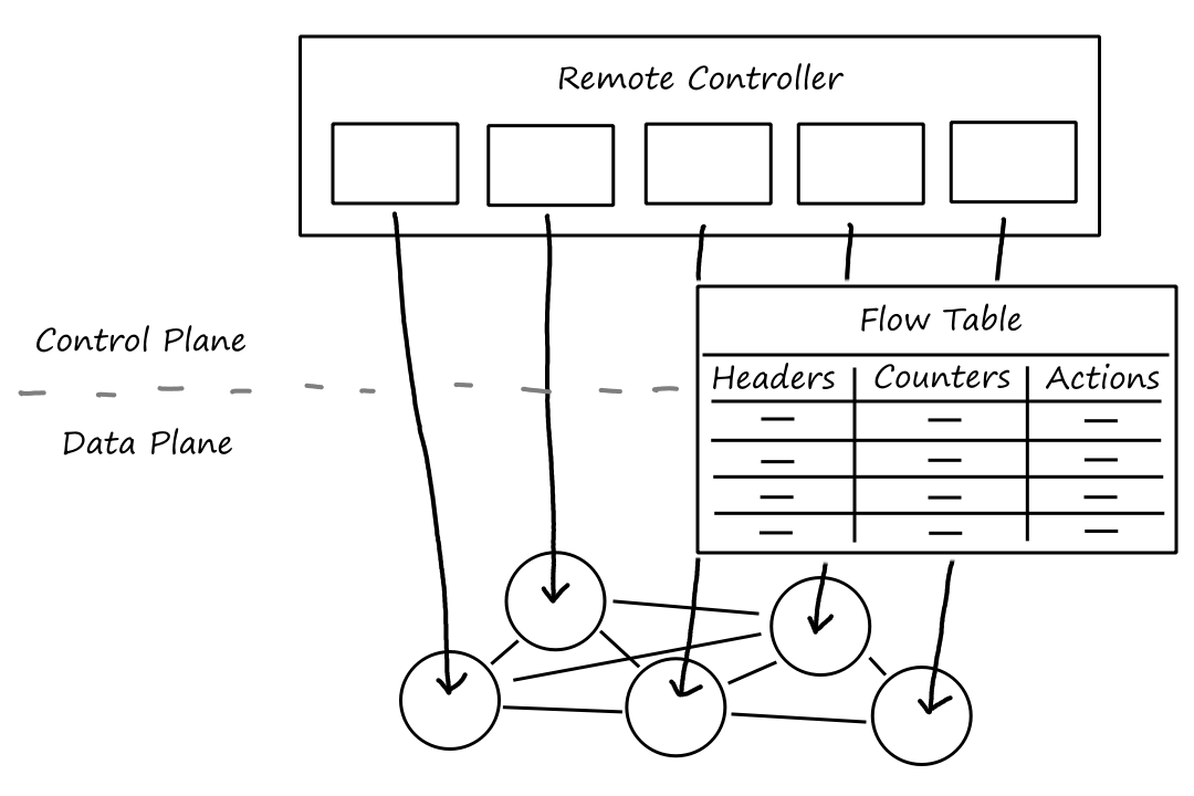
Match
There are `12` things that are checked for matching:
- Ingress port (the ID of the router's input port)
- Source MAC address (link layer)
- Destination MAC address (link layer)
- Ethernet type (link layer)
- VLAN ID (link layer)
- VLAN priority (link layer)
- Source IP address (network layer)
- Destination IP address (network layer)
- IP Protocol field (network layer)
- IP TOS field (network layer)
- TCP/UDP source port (transport layer)
- TCP/UDP destination port (transport layer)
There is typically not a rule for every single possible combination of values for all of these things. Some flow table entries can use wildcards. For example, a rule that matches an IP address of 128.119.*.* means that any IP address that starts with 128.119 will match that entry.
Action
There can be multiple actions to perform for a certain packet. The packet switch can forward the packet to an output port, drop the packet, or modify the packet-header fields before forwarding it.
OpenFlow Examples of Match-plus-action in Action
Suppose we have a network with `6` hosts and `3` packet switches, each with `4` interfaces.

Simple Forwarding
Let's say there is a packet from h5 (or h6) that is going to h3 (or h4), and it's cheaper to go through s1. This could be s1's flow table:
| Match | Action |
|---|---|
| Ingress Port = 1; Source IP = 10.3.*.*; Destination IP = 10.2.*.* | Forward to 4 |
This could be s3's flow table:
| Match | Action |
|---|---|
| Source IP = 10.3.*.*; Destination IP = 10.2.*.* | Forward to 3 |
And this could be s2's flow table:
| Match | Action |
|---|---|
| Ingress Port = 2; Destination IP = 10.2.0.3 | Forward to 3 |
| Ingress Port = 2; Destination IP = 10.2.0.4 | Forward to 4 |
Load Balancing
Let's say packets from h3 and h4 are going to h2. But to reduce network congestion, we want the packets to travel through different links. This could be s2's flow table:
| Match | Action |
|---|---|
| Ingress Port = 3; Destination IP = 10.1.0.2 | Forward to 2 |
| Ingress Port = 4; Destination IP = 10.2.0.2 | Forward to 1 |
So h3's packet would take the direct route from s2 to s1, while h4's packet would go from s2 to s3 to s1.
Firewalling
Let's say s2 only wants to receive packets from s3. This could be s2's flow table:
| Match | Action |
|---|---|
| Source IP = 10.3.*.*; Destination IP = 10.2.0.3 | Forward to 3 |
| Source IP = 10.3.*.*; Destination IP = 10.2.0.4 | Forward to 4 |
Note that there are no rules for Source IP = 10.1.*.*, so packets coming from s1 would be dropped.
Now to the link layer!
Introduction to the Link Layer
We'll call a device that runs a link-layer protocol a node. And the communication channels that connect the nodes are called links. A node encapsulates a datagram in a link-layer frame and transmits the frame into the link. The job of the link layer is to transfer frames from one node to another.
Suppose we are traveling and a travel agent plans for us to take a bus from A to B, a plane from B to C, and a train from C to D. In this analogy, we would be a datagram, each transportation segment would be a link, the mode of transportation would be a link-layer protocol, and the travel agent would be a routing protocol.
Where Is the Link Layer Implemented?
Most of the link layer is implemented on a chip called the network adapter, which is also sometimes called a network interface controller. The network adapter is the one that does the encapsulation, and it also does error detection.
Some of the link layer is implemented in software as well. The software handles error conditions and passes datagrams up to the network layer.
Error-Detection and -Correction Techniques
As frames move across links, some of their bits may get flipped. So the receiver on the other side of the link has to perform error detection. However, the error-detection techniques available are not completely reliable; there may still be undetected bit errors, but this is rare.
Let `D` denote the data that is being sent. At the sending node, `D` is combined with error-detection and -correction bits denoted as `EDC`. Let `D'` and `EDC'` be the result of the frame moving across the link. Given only `D'` and `EDC'`, the receiver has to check if `D'` is the same as `D`.
A larger number of `EDC` bits lowers the probability of undetected bit errors (by allowing for more sophisticated error-detection techniques), but results in a larger computation and transmission overhead.
Parity Checks
Suppose `D` has `d` bits. The sending node will add a single parity bit such that the total number of `1`s is even (or odd in an odd parity scheme). The receiving node will then count the number of `1`s. If an even parity scheme is used, then if the receiver counts an odd number of `1`s, then it knows there is a bit error. If there are an even number of `1`s, then it thinks there are no errors. (Note that it's possible for bits to be flipped in a way such that there are still an even number of `1`s. In this case, there would be an undetected bit error.)
For example, consider `d` data bits: `0 1 1 1`. There are an odd number of `1`s, so the sender will add a `1` as the parity bit.
`ubrace(0 1 1 1)_text(d bits) ubrace(1)_text(parity bit)`
Now let's look at two-dimensional parity. Suppose the `d` bits are divided into `i` rows and `j` columns.
`[[d_(1,1),...,d_(1,j)],[d_(2,1),...,d_(2,j)],[vdots, ddots, vdots],[d_(i,1),...,d_(i,j)]]`
The parity will be computed for each row and column, so there will be `i+j+1` parity bits.
For example, suppose the `d` bits look like this:
`[[1,0,1,0,1],[1,1,1,1,0],[0,1,1,1,0]]`
Suppose that none of the bits got flipped. Then the top-left half is the result.
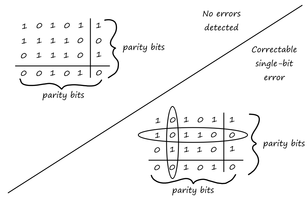
Now suppose the bit in the second row and second column got flipped. Then the bottom-right half is the result. There an odd number of `1`s in that row and column, so we can tell exactly where the error occurred. Actually, we can go even further and correct the error by changing the `0` to a `1`. The ability to detect and correct errors is called forward error correction (FEC).
It is also possible for the parity bits to get flipped.
Checksum
Back in the transport layer, we saw the checksumming algorithm that UDP uses. The Internet checksum is pretty much the same: the sender will divide the data into `16`-bit integers, get the sum, and perform `1`s complement to calculate the checksum. When the receiver gets the data, it will divide the data into `16`-bit integers, get the sum, and add that sum to the checksum that the sender computed. If all the bits are the same, then no errors were detected. If some of the bits are different, then there was an error.
Checksumming is a lightweight operation, but it's also a fairly weak error-detection technique. It's used in the transport layer though because the transport layer is implemented in software. Using software to run complicated algorithms can take a long time, so it's better to have software running a fast operation.
Since error detection in the link layer is implemented in hardware, stronger, more complex algorithms can be used.
Cyclic Redundancy Check (CRC)
The error detection that is performed at the link layer is based on cyclic redundancy check (CRC) codes.
Before doing anything, the sender and receiver first have to agree on a special number, which we'll call a generator, denoted as `G`. The leftmost bit of `G` must be `1`. Then the sender will append `r` bits (all denoted as `R`) to `D` such that the resulting `d+r` bits are divisible by `G`. So the receiver will divide the `d+r` bits by `G` and if the remainder is not zero, then it knows there was an error.
All CRC math operations are done in modulo-`2` arithmetic without carries in addition and borrows in subtraction. This means that `1+1=0` and `0-1=1`. As a result, addition and subtraction are the same. For example,
`1011-0101=1110=1011+0101`
`1001-1101=0100=1001+1101`
This also happens to be equivalent to the XOR operator, where it's `1` if both bits are different and `0` if both bits are the same. So adding/subtracting in modulo-`2` is the same as performing XOR.
In binary arithmetic, multiplying a number by `2^k` shifts the bits to the left `k` times. For example, consider `5*4=20`. `5` in binary is `101` and `20` in binary is `10100`. In this case, `4=2^k implies k=2`, and we can see that `10100` is indeed `101` shifted to the left `2` times.
So if we multiply `D` by `2^r`, `D` will be shifted to the left `r` times. Then if we XOR `D*2^r` with `R`, we'll end up with the `d+r` bit pattern.
So once the sender and receiver know what `G` is, the sender has to pick `R` such that the `d+r` bits is a number divisible by `G`. But how?
First, the `d+r` bits can be represented as `D*2^r text( XOR ) R`. In order for it to be divisible by `G`, there has to exist an `n` such that
`D*2^r text( XOR ) R = nG`
If we XOR (add modulo-`2` without carry) `R` to both sides, we get
`D*2^r = nG text( XOR ) R`
Let's try to express `D*2^r` as a product involving `G`. Consider for a moment what happens when we divide `D*2^r` by `G`. The result will be some number plus a remainder. And remember that "plus" is the same as "XOR" in CRC math.
`D*2^r = nG text( XOR ) R`
`text(some number)*G text( XOR a remainder) = nG text( XOR ) R`
This means that the remainder is `R`. So we've found `R`, which is the question we wanted to answer! `R` is the remainder of `(D*2^r)/G`.
Suppose `D=101110`, `G=1001`, and `r=3`. To find `R`, we divide `D*2^r` by `G`.

Multiple Access Links and Protocols
There are two types of network links: point-to-point links and broadcast links. A point-to-point link has one node on each end of the link. A broadcast link can have multiple sending and receiving nodes on each end of the link. So when one node transmits a frame, all the nodes on the same channel receive a copy of it.
However, when multiple nodes can send and receive at the same time, things can get messy. This is referred to as the multiple access problem. If more than two nodes transmit frames at the same time, then the other nodes will receive them at the same time. The frames will collide with each other and get all mixed up.
To prevent collisions, there are multiple access protocols that coordinate the transmission of the nodes. Ideally, the protocols should satisfy these conditions:
- when one node is sending, it has a throughput of `R` bits per second (where `R` is the rate of the channel)
- when `M` nodes are sending, each of them has an average (not instantaneous) throughput of `R/M` bps
- the protocol is decentralized so that there is no master node (and thus no single point of failure)
- the protocol is simple and inexpensive
Channel Partitioning Protocols
Remember time-division multiplexing (TDM) and frequency-division multiplexing (FDM)? They're two ways to divide a broadcast channel's bandwidth among all the nodes sharing that channel.
TDM divides time into time frames, which are then further divided into time slots. If there are `N` nodes, then each time frame will be divided into `N` slots, one for each node. So a node will only send data when its turn arrives.
TDM prevents collisions and guarantees each node gets `R/N` throughput during each frame time. This guarantee can also be a drawback though. A node gets at most `R/N` throughput, even if it is the only node that has data to send. In addition, a node has to wait for its turn to send data, even if it is the only node with data to send.
FDM divides the channel into `N` different frequencies, each with a bandwidth of `R/N`. In this case, a node can send data at any time, but it is still limited to at most `R/N` bps, even if it is the only node with data to send.
A third channel partitioning protocol is code division multiple access (CDMA). A unique code is assigned to each node, and each node uses its code to encode the data it sends. The codes can be chosen in such a way that all the nodes can transmit at the same time and their respective receivers won't get mixed up, assuming the receiver knows the sender's code.
Random Access Protocols
In random access protocols, nodes always transmit at `R` bits per second and wait for some random time when a collision occurs. When a collision occurs, the nodes involved repeatedly send their frames until they get through with no collisions. Of course, if they all repeatedly send at the same time, collisions will keep happening. So each node waits a random delay before retransmitting.
Slotted ALOHA
In slotted ALOHA, time is divided into slots like in TDM. Unlike in TDM, all nodes get to utilize the full bandwidth and send at the same time. At each time slot, each node randomly decides whether it will send or wait until the next slot.
We'll assume that
- all frames have `L` bits
- the length of a slot is the time it takes to transmit one frame (i.e., a slot is `L/R` seconds long)
- nodes start to transmit only at the beginning of slots
- each node knows when the slots begin (i.e., they're synchronized)
- all the nodes involved in a collision detect the collision before the slot ends
Slotted ALOHA is decentralized since each node detects collisions and independently decides when to transmit. And besides needing the nodes to be synchronized, it's a pretty simple protocol.
However, it's not that efficient. When there are multiple active nodes (nodes that have frames to send), some of the slots will have collisions and be "wasted". There's also a chance that none of the nodes decide to transmit during a time slot, resulting in an unutilized slot.
A successful slot is a slot in which exactly one node transmits. The efficiency of a slotted multiple access protocol is the fraction of successful slots over time when there are a lot of active nodes.
Suppose that each node tries to transmit a frame in each slot with probability `p`. A slot is successful if one node transmits and the other `N-1` nodes don't. The probability of this is `p(1-p)^(N-1)`. The probability that any of the `N` nodes succeeds is `Np(1-p)^(N-1)`.
So when there are `N` active nodes, the efficiency is `Np(1-p)^(N-1)`. The math gets a little funky, but it turns out that the maximum efficiency is `1/e~~0.37` (and the probability that achieves this maximum efficiency is `p=1/N`).
This means that when there are a lot of active nodes, only `37%` of the slots will be successful. A channel capable of transmitting a frame at `100` Mbps will effectively only have a successful throughput of `37` Mbps in the long run.
ALOHA
In pure ALOHA, there are no time slots (so the nodes don't need to be synchronized). Whenever a node receives a frame, it just transmits the frame right away. If there is a collision, the node will retransmit with probability `p` or wait for some time with probability `1-p`.
With no time slots to synchronize the sending, the likelihood of collisions increases greatly. But how bad is it?
Suppose node `i` begins transmitting a frame at time `t_0`. In order for this frame to be successfully transmitted, no other frames can start to be transmitted between `t_0-1` and `t_0`. This happens with probability `(1-p)^(N-1)`.

In addition, no other frames can start to be transmitted between `t_0` and `t_0+1`. This also happens with probability `(1-p)^(N-1)`.
So the probability that the frame is successfully transmitted is `p*(1-p)^(N-1)*(1-p)^(N-1)=p(1-p)^(2(N-1))`. After some of the funky math again, it turns out that the maximum efficiency is `1/(2e)`, which is half the efficiency of slotted ALOHA.
Carrier Sense Multiple Access (CSMA)
Naturally, it makes sense to have the nodes check the channel before transmitting. If the channel is not being used by any other nodes, then the node can begin transmitting. If the channel is busy, then the node should wait and then check again later. This is called carrier sensing. From a node's perspective, a channel is busy if it can detect a signal on the channel from another node.
However, it's still possible for collisions to happen. Let's say node `A` starts transmitting a frame at time `t_0`. Suppose, for some reason, that it takes a lot of time for that node's bits to propagate along the channel (channel propagation delay). Let's say node `B` checks the channel at time `t_1` and the bits from node `A` haven't reached `B` yet. `B` will think that the channel is empty and start transmitting. So now there are two frames being transmitted, resulting in a collision.

Carrier Sense Multiple Access with Collision Detection (CSMA/CD)
While a node is transmitting, if it detects that another node is transmitting, then the node will stop transmitting and wait before trying again. This is collision detection. Having collision detection prevents damaged frames from being sent.
So how long should the nodes wait if they detect a collision? If the waiting interval is large, but the number of collisions was small, then the channel will be idle for quite some time. On the other hand, if the waiting interval is small, but the number of collisions is large, then it's likely some of the nodes will wait the same amount of time as each other and collide again.
The binary exponential backoff algorithm is used to solve this problem. When a node transmits a frame that has already had `n` collisions, that node waits for a random time from `0` to `2^n-1`. So the more collisions the frame has had, the longer it potentially has to wait before being retransmitted.
- After `1` collision: `{0,1}`
- After `2` collisions: `{0,1,2,3}`
- After `3` collisions: `{0,1,2,3,4,5,6,7}`
- After `10` collisions: `{0,1,2,...,1023}`
Let `K` be the random time that is picked from `{0,1,2,...,2^n-1}`. For Ethernet, the maximum value of `n` is `10`, and the actual amount of time a node waits is `K*512` bit times. `512` bit times is the amount of time needed to send `512` bits into the Ethernet. For a `100` Mbps Ethernet, `512` bit times is `5.12` microseconds.
CSMA/CD Efficiency
The efficiency of CSMA/CD is the fraction of time during which frames are successfully transmitted when there are lot of active nodes.
Let `d_text(prop)` be the maximum time it takes signal energy to propagate between any two nodes. Let `d_text(trans)` be the time to transmit a maximum-size frame. The efficiency turns out to be
`1/(1+(5d_text(prop))/d_text(trans))`
Note that as `d_text(prop) rarr 0`, the efficiency approaches `1`. This makes sense because if nodes can quickly tell when the channel is busy, they can wait to transmit and prevent a collision (or stop their transmission if they were already transmitting and prevent wasted time).
Also, as `d_text(trans) rarr oo`, the efficiency approaches `1`. In this case, the frame is very large, so it will take a while for the node to transmit it. The longer this takes, the less likely it is for other nodes to cause collisions (since the time to transmit will likely cancel out the effect of channel propagation delay). So all of this time will be counted towards successful transmission.
For the channel partitioning protocols:
- the channel is efficient and fair at high loads
- the channel is inefficient at low loads
- when there is only one active node, it only has a throughput of `1/N`
For the random access protocols:
- the channel is efficient at low loads
- when there is only one active node, it can fully utilize the channel
- there are collisions at high loads
Taking-Turns Protocols
As mentioned earlier, when one node is active, it should ideally have a throughput of `R`. And when `M` nodes are active, they all should ideally have a throughput of `R/M`. Random access protocols satisfy the first property but not the second. So taking-turns protocols were developed to try to achieve both.
Polling Protocol
In the polling protocol, a central controller node polls each of the other nodes one at a time. If the current node being polled has data to send, then it will be allowed to send. If the current node has no data to send, then the controller node will poll the next node.
Since only one node is sending at a time, there are no collisions. There are also not a lot of empty slots since the controller node immediately polls the next node. So this is pretty efficient.
However, there is a polling delay from the controller node to the other nodes. Also, the whole thing fails if the controller node fails.
Token-Passing Protocol
Instead of a controller node that decides when the nodes get to send, there is a token that is passed around in some fixed order. When the node gets the token, it gets to send.
While this is also decentralized and efficient, there can be problems with passing the token. For example, if one node fails, then the whole thing fails since the token will not get past that failed node.
Switched Local Area Networks
A link-layer switch operates at the link layer, so they switch link-layer frames and don't recognize network-layer addresses. This is different from a layer-3 (network layer) packet switch.
Link-Layer Addressing and ARP
MAC Addresses
In addition to having an IP address, network interfaces also have a link-layer address. LAN address, physical address, and MAC address are all terms for a link-layer address.
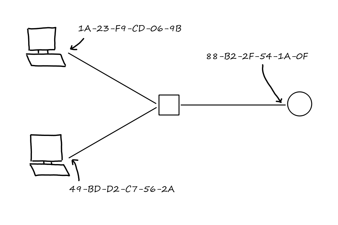
The square is a link-layer switch and the circle is a router.
Only the interfaces on hosts and routers have link-layer addresses. For link-layer switches, their adapters that connect to hosts and routers do not have link-layer addresses. This is because, at the network layer, hosts or routers set the destination of the datagram to another host or router, not to a link-layer switch.
A MAC address is `6` bytes long and are represented as six pairs of hexadecimal numbers.
Since a MAC address has `48` bits, there are `2^48` possible MAC addresses. Interestingly, no two adapters have the same MAC address. So how does one company manufacturing adapters make sure that their adapters don't have the same addresses as other adapters from another company? The answer is similar to the way ISPs give out IP addresses to companies. In this case, IEEE manages the MAC address space, and companies purchase a chunk of the address space (`2^24` addresses). IEEE fixes the first `24` bits and lets the company choose the last `24` bits.
While IP addresses are hierarchical (they have a network part and host part) and change when connected to a different network, MAC addresses are not hierarchical and always stay the same regardless of which network the device is connected to.
When an adapter wants to send a frame, it puts the destination adapter's MAC address into the frame and sends the frame into the LAN. When an adapter receives a frame, it checks to see if the destination MAC address in the frame matches its own MAC address. If it matches, the adapter extracts the datagram from the frame and passes it up to the network layer. If the sending adapter wants to send a frame to all adapters on the LAN, it will use a special MAC broadcast address (all `1`s, which is FF-FF-FF-FF-FF-FF in hexadecimal) as the destination.
Address Resolution Protocol (ARP)
The Address Resolution Protocol (ARP) is used to translate between network-layer addresses and link-layer addresses.
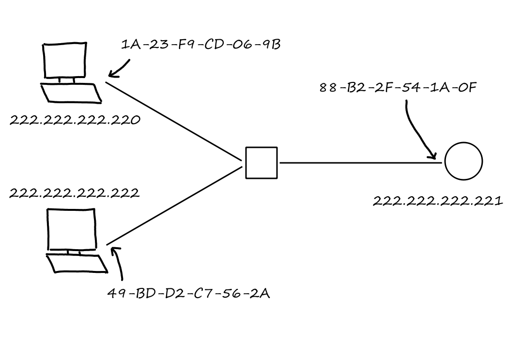
The IP addresses are shown in dotted-decimal notation and the MAC addresses are shown in hexadecimal notation.
Suppose 222.222.222.220 wants to send an IP datagram to 222.222.222.222. In order for this to happen, the source has to give its adapter the IP datagram and the destination MAC address for 222.222.222.222. But how does the source know what the MAC address of 222.222.222.222 is?
This is where ARP comes in. An ARP module in the sending host looks up the IP address in an ARP table and returns the corresponding MAC address.
| IP Address | MAC Address | TTL |
|---|---|---|
| 222.222.222.221 | 88-B2-2F-54-1A-0F | 13:45:00 |
ARP only resolves IP addresses for host and router interfaces on the same subnet.
But what happens if an IP address doesn't exist yet in an ARP table? For example, 222.222.222.220 wants to send an IP datagram to 222.222.222.222, but the receiver's MAC address is not in the sender's ARP table. First, the sender will send an ARP packet to the MAC broadcast address asking all the hosts and routers for their MAC address if their IP address is 222.222.222.222. Then, 222.222.222.222 will respond to 222.222.222.220 with its MAC address.
ARP is a plug-and-play protocol. The ARP table gets built automatically without needing any human intervention.
An ARP packet is encapsulated within a link-layer frame. That is, an ARP packet is not a link-layer frame. However, an ARP packet has link-layer fields like a link-layer frame does.
Sending a Datagram off the Subnet
So far, we've seen how ARP works for hosts on the same subnet. But what if a host wants to send a datagram to another host that is on a different subnet? Suppose there are two subnets connected by a router.
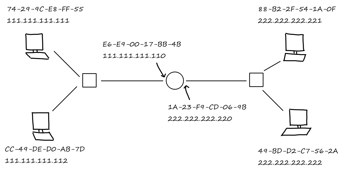
What happens when 111.111.111.111 wants to send a datagram to 222.222.222.222? Well, in order to get to 222.222.222.222, the datagram would have to go through the router. So the sender puts 222.222.222.222 as the destination IP address and E6-E9-00-17-BB-4B (the router's MAC address) as the destination MAC address. (And the router's MAC address is obtained via ARP.) When the router gets the frame, it extracts the datagram and passes it up to the network layer.
Now the router has to determine which output link to forward the datagram to. As we saw before, this is done by looking at the forwarding table. Once it knows where to forward the datagram, the router's adapter encapsulates the datagram into a frame and sends the frame to the receiver. Again, the MAC address of the receiver is obtained via ARP.
Ethernet
Ethernet is the most dominant wired LAN technology. It was the first widely deployed high-speed LAN, and it was simpler, cheaper, and faster than other LAN technologies.
Most, if not all, LANs with Ethernet are set up using a star topology where there is a switch at the center.
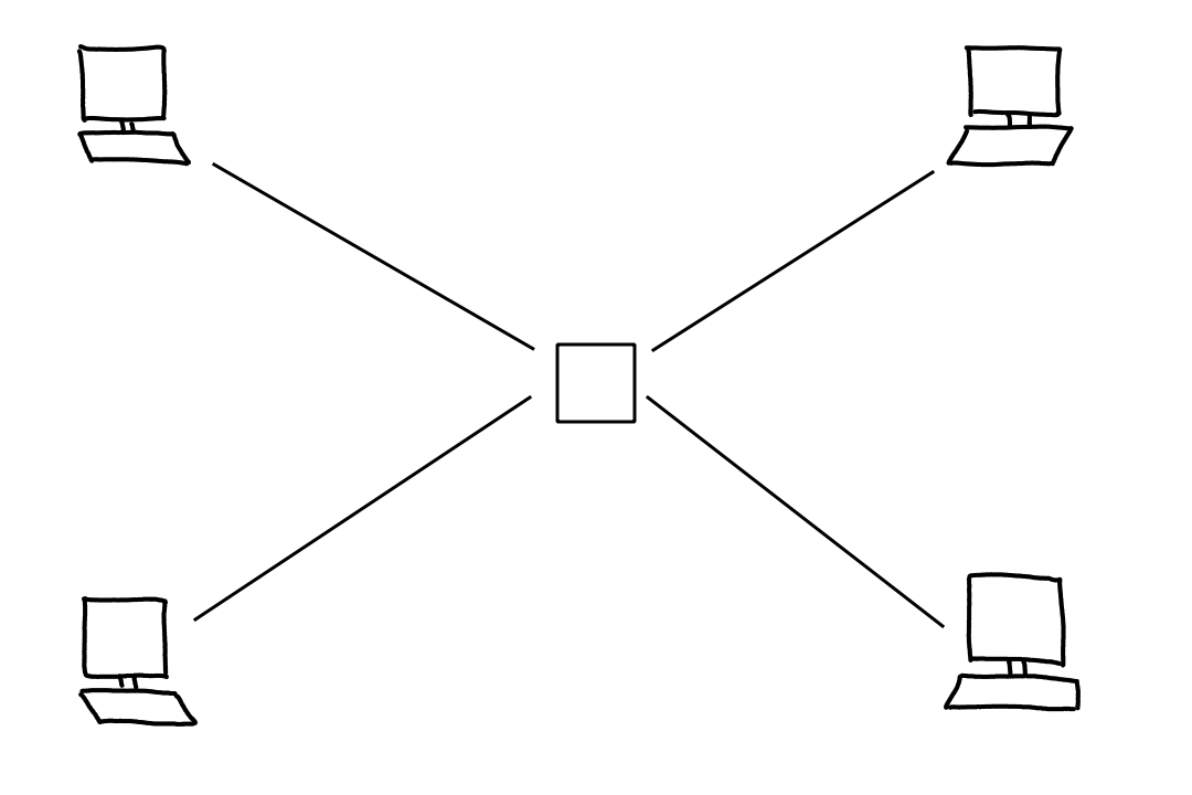
Ethernet Frame Structure
The following are included in an Ethernet frame:
- data field (`46` to `1500` bytes)
- contains the IP datagram
- destination MAC address (`6` bytes)
- source MAC address (`6` bytes)
- type field (`2` bytes)
- used to specify which network-layer protocol is receiving this frame
- cyclic redundancy check (`4` bytes)
- used to detect bit errors (see the Cyclic Redundancy Check (CRC) section)
- preamble (`8` bytes)
- used to "wake up" the receiving adapters, i.e., sync their clocks to the sender's clock
- first `7` bytes is 10101010; last byte is 10101011
Ethernet is connectionless and unreliable, kinda like UDP. But if the transport layer being used is TCP, then there won't be data loss.
Link-Layer Switches
A switch receives incoming link-layer frames and forwards them onto outgoing links, similar to what routers do for datagrams. Switches are transparent to hosts and routers, meaning that hosts and routers are not aware of their existence. This goes back to the reason why the adapters on link-layer switches do not have link-layer addresses mentioned earlier.
Forwarding and Filtering
Forwarding is determining which interface the frame should be transferred to (and moving the frame). Filtering is determining whether a frame should be forwarded or dropped. Both of these actions are based on a switch table.
| Address | Interface | Time |
|---|---|---|
| 62-FE-F7-11-89-A3 | 1 | 9:32 |
| 7C-BA-B2-B4-91-10 | 3 | 9:36 |
An entry in the switch table contains a MAC address, the interface that leads to that MAC address, and the time that the entry was created. Whenever a frame arrives at a switch, the switch adds the frame's source address and the interface it came from to the switch's switch table.
If a frame arrives at a switch and there is no entry in the switch table for the frame's destination address, then the switch broadcasts the frame to all of the switch's other interfaces.
Suppose a frame with destination address 62-FE-F7-11-89-A3 arrives at switch `A` from interface 1. Then the switch will filter (discard) the frame.
Wait, but how does a frame with destination address 62-FE-F7-11-89-A3 come from interface 1? After all, the frame should've been sent to interface 1 because the switch table said to do that.
Suppose that when switch `A` received the frame, it didn't have 62-FE-F7-11-89-A3 in its switch table yet. So switch `A` broadcasts the frame to all its other interfaces. Let's say its interface 1 is connected to another switch `B`, which also doesn't have 62-FE-F7-11-89-A3 in its switch table. When `B` gets the frame, it will also broadcast the frame to all its other interfaces, including the one that leads back to `A`.
Let's say that a frame from 62-FE-F7-11-89-A3 is already headed to switch `A` and arrives at `A` before `B` performs its broadcast. Now, `A` will have 62-FE-F7-11-89-A3 in its switch table. And by the time `B`'s broadcast reaches `A`, `A` will already have 62-FE-F7-11-89-A3 in its switch table.
Self-Learning
A switch is called self-learning because its switch table is built automatically.
- Initially, the switch table is empty.
- When the switch receives a frame on an interface, the switch puts the frame's source address and the interface it came on in the switch table.
- After some time (aging time), if no frames are received from an address, then the entry with that address is deleted from the table.
Switches are plug-and-play devices; once they're physically connected to the network, they just work. Switches are also full-duplex, so any switch interface can send and receive at the same time.
Properties of Link-Layer Switching
- No collisions: Switches buffer frames and only transmit one frame at a time.
- Heterogeneous links: A switch can have multiple types of links that have different speeds.
- Management: A switch can automatically disconnect a malfunctioning adapter.
Switch Poisoning
Recall that when a switch receives a frame and the destination address isn't in its switch table, the switch broadcasts the frame to everyone. This is one way an attacker can obtain (sniff) a frame that wasn't intended to be sent to the attacker.
To effect this, the attacker can send a bunch of packets with fake MAC addresses to a switch. As a result, the switch will fill up its switch table with these fake addresses, preventing real MAC addresses from being put in the table. And since those real addresses aren't in the table, the frames for those addresses will be broadcasted.
Switches Versus Routers
While both routers and switches are store-and-forward packet switches, routers are layer-3 packet switches (so they forward using IP addresses) and switches are layer-2 packet switches (so they forward using MAC addresses). When setting up a network, network admins have to decide whether to use routers or switches as the interconnection devices between hosts.
Switches are plug-and-play and have relatively high filtering and forwarding rates since they only have to process frames up through layer 2.
But to prevent broadcast frames from being repeatedly cycled through the network, the topology of a switched network is restricted to a spanning tree. Switches are also susceptible to broadcast storms in which one or more hosts repeatedly transmits broadcast frames, bringing down the whole network.
Since network addresses are hierarchical and there is a hop limit field in datagrams, datagrams don't have a chance to repeatedly get cycled through the network. So the topology with routers is flexible. Routers also have firewall protection against broadcast storms.
However, routers are not plug-and-play; they need their IP addresses to be configured. Also, routers have to process datagrams up through layer 3, so they have slower processing times.
Typically, smaller networks use just switches, and larger networks use routers and switches. Since larger networks have more links for data to traverse, they benefit from the routers' capability to provide optimal routes.
Virtual Local Area Networks (VLANs)
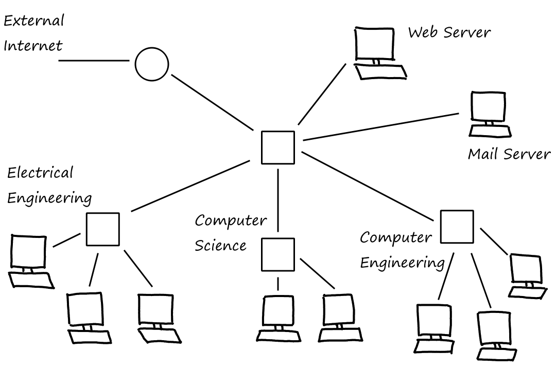
This is an example of a switched LAN network for a school. There are three departments (EE, CS, CE), connected to a network of `4` switches and `1` router. However, there are several issues with this setup.
There is no traffic isolation. Broadcast traffic, like ARP and DHCP messages or frames whose destination address is not in the switch table yet, gets transmitted across the entire network. Limiting the traffic to just its intended group would increase performance and provide more security and privacy.
One way to have traffic isolation is to replace the center switch with a router. (See the Routing Policy section.)
The switches are being used inefficiently. If there were `10` departments instead of `3`, then `10` first-level switches would be used. This becomes more inefficient if the departments are small.
It's hard to manage users. If someone moves from one group to another, the cables must be reconfigured to connect that person to a different switch.
These three problems can be solved by virtual local area networks (VLANs). In this setup, multiple virtual local area networks are created on top of a single physical local area network. In a port-based VLAN, the switch's ports (interfaces) are divided into groups, where each group represents a VLAN.
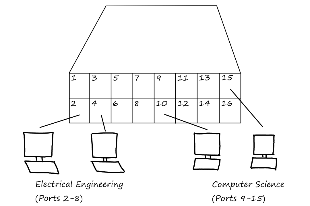
The switch can be configured so that traffic from one port stays within that port's group. This provides traffic isolation.
There is a single switch replacing all those switches in the network above. So this one switch is being really efficient.
If one user moves to a different group, then the port that the user is connected to can be reconfigured to belong to another VLAN.
But what if someone from the EE department wants to communicate with someone in the CS department? One way to allow this is to reserve one port that is not being used by any VLANs and configure that port to belong to both the EE and CS departments. That port would then be used by an external router. So an IP datagram from the EE department would first go from the EE VLAN to the router. Then the router would forward the datagram to the CS VLAN.
But let's suppose that some faculty are in a different building entirely, so that they're not connected to the same switch as everyone else. How can people in these two buildings communicate with each other?
We could connect the two switches by VLAN trunking. One port on each switch (trunk port) is reserved for a trunk link to connect the two switches together. Frames that travel across the trunk link will have a VLAN tag in the header so that the switch knows which VLAN the frame should be sent to.
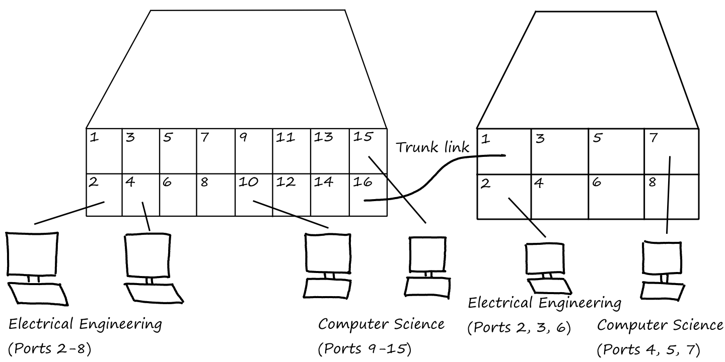
Link Virtualization: A Network as a Link Layer
A link between two nodes can sometimes be a whole network.
But how can those two nodes be "connected by a link" when there are a whole network of links between them? They're neighbors in the sense that they are next-hop routers for each other.
Multiprotocol Label Switching (MPLS)
MPLS is a routing protocol that forwards datagrams based on a fixed-length label instead of IP addresses. This makes forwarding faster by making the lookup faster.
Frames that are handled by MPLS-capable routers (a.k.a. label-switched routers) have an MPLS header that contain the MPLS label. With this header, MPLS-capable routers don't need to extract the destination IP address and perform a lookup of the longest prefix match in the forwarding table.
MPLS is considered a layer-2.5 protocol.
These MPLS-enhanced frames can only be sent to and from MPLS-capable routers. However, it's also possible for MPLS-capable routers and standard IP routers to be connected to each other. So how does this work?
As we saw before, routers continuously send advertisements to other routers (see Advertising BGP Route Information). Through these advertisements, MPLS-capable routers can find out if their neighbors are also MPLS capable. A standard router will forward a frame to an MPLS-capable router just like it would any other router. But if an MPLS-capable router has an MPLS-capable neighbor, it will add that MPLS header to the frame and forward it. Thus, this faster forwarding will occur as long as there is an MPLS-capable neighbor. Once there is no longer an MPLS-capable neighbor, the last MPLS-capable router will take out the MPLS header so that the next standard router won't get confused.
This is very similar to tunneling for integrating IPv6 routers with IPv4 routers. (See the Transitioning from IPv4 to IPv6 section.)
Let's look at an example of a setup. Routers `R1`, `R2`, `R3`, and `R4` are MPLS capable while routers `R5` and `R6` are standard IP routers. Router `R1` advertises to `R2` and `R3` that it can reach destination `A` if it receives a frame with an MPLS label of `6`.
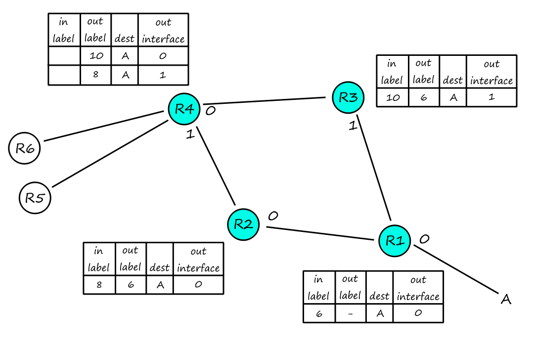
After all the routers advertise to each other, `R4` learns of two paths to reach `A`. It can either send it to `R3` or `R2` since both of them can reach `R1`, which can reach `A`.
If these were all standard routers, then BGP's route-selection algorithm would've only provided one least-cost path. But in this case, multiple paths exist and any of them can be used. While faster forwarding is nice, this is the true advantage of MPLS; taking advantage of this capability is one form of traffic engineering.
MPLS is used to implement virtual private networks (VPNs).
Data Center Networking
Companies like Google, Microsoft, and Amazon have large data centers to provide their contents and services to us. These data centers are connected to the Internet, and they themselves are complex computer networks, called data center networks.
Data centers provide Web pages, search results, email (basically data from the Internet); they provide extra computational resources for data processing tasks; and they provide cloud computing services.
Data Center Architectures
The computers in a data center are the hosts, which are also called blades. They are stacked in racks, with each rack having about `20` to `40` blades. At the top of the rack, there is a Top of Rack (TOR) switch that connects all the hosts in the rack with each other and with the other switches in the data center.
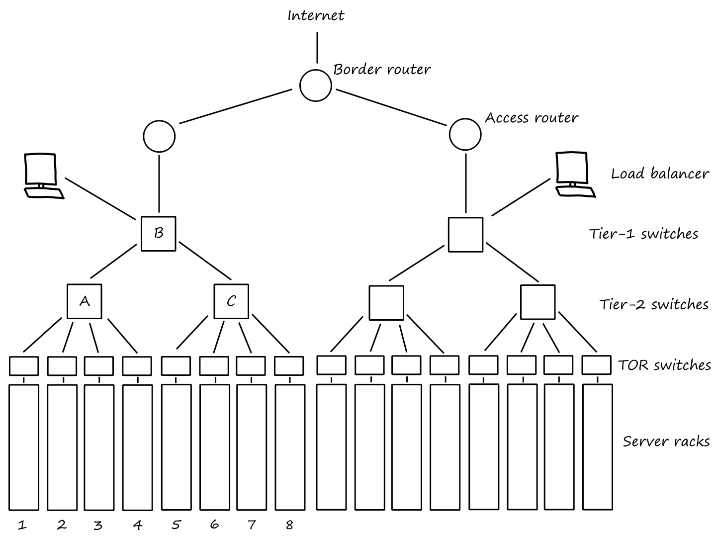
To handle traffic to/from outside the data center, there are border routers that connect the data center network to the Internet.
Load Balancing
A data center will have a load balancer to distribute requests evenly across different hosts.
A load balancer can be seen as a "layer-4 switch" since it forwards requests based on the destination port and IP.
Hosts are given an internal IP address that is local to the data center and an external IP address that the outside Internet can communicate with. The load balancer performs a NAT-like function by converting between these addresses when they send/receive data to/from these hosts.
Hierarchical Structure
One problem data centers have to deal with is limited host-to-host capacity. Suppose that each host connects to its TOR switch with a `10` Gbps link and that the switches connect to each other with `100` Gbps links.
Hosts in the same rack can communicate with each other at the full `10` Gbps rate. But hosts in different racks communicating with each other can have a more limited rate.
Suppose that `10` hosts in rack `1` communicate with `10` hosts in rack `5`; `10` hosts in rack `2` communicate with `10` hosts in rack `6`; `10` hosts in rack `3` communicate with `10` hosts in rack `7`; `10` hosts in rack `4` communicate with `10` hosts in rack `8`. So there are `40` flows crossing the `A`-to-`B` link (and the `B`-to-`C` link). If the link divides its capacity among the `40` flows, then each flow will only get `100/40=2.5` Gbps.
Of course, using higher-rate switches and routers is an option, but that gets very expensive.
Another way to deal with this is to try and group co-related services and data as close to each other as possible (ideally in the same rack). But this can only go so far.
Perhaps the most ideal way to deal with this is to introduce more links. So the TOR switches could be connected to multiple tier-2 switches, and the tier-2 switches can be connected to multiple tier-1 switches. This provides increased capacity and increased reliability since there are now multiple paths between switches.
A Day in the Life of a Web Page Request
Let's look at what happens when we connect our laptop to our school's network and go to google.com. Let's say the laptop is connected to the school's network by an Ethernet cable to an Ethernet switch, which is connected to a router. Then the router is connected to the school's ISP, which in this case, is comcast.net. The ISP is also providing the DNS service for our school.
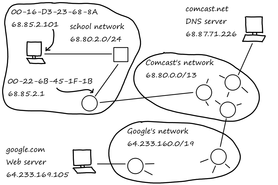
Getting Started: DHCP, UDP, IP, and Ethernet
First, our laptop needs an IP address, and this can be obtained using the DHCP protocol. We'll assume that the router is running the DHCP server.
- Our laptop creates a DHCP request message and puts this message in a UDP segment. The UDP segment is put in an IP datagram with a broadcast destination address (255.255.255.255) and a source IP address of 0.0.0.0.
- The IP datagram is put in an Ethernet frame, which has a broadcast destination MAC address (FF-FF-FF-FF-FF-FF) so that it can reach the DHCP server (running in the router).
- The frame gets sent to the Ethernet switch, which broadcasts the frame to all of its outgoing ports.
- The router receives the frame and extracts the IP datagram from it. Since the destination IP address is the broadcast address, the router will process this datagram and demultiplex the datagram's payload to UDP. UDP then sends the DHCP request message to the DHCP server.
- Let's say the DHCP server can allocate IP addresses in the CIDR block 68.85.2.0/24, and that the IP address that is chosen is 68.85.2.101. The DHCP server creates a DHCP ACK message containing this IP address along with the IP address of the DNS server (68.87.71.226), the IP address of the default gateway router (68.85.2.1), and the subnet block (68.85.2.0/24) (a.k.a. network mask). The DHCP message is put inside a UDP segment, which is put inside an IP datagram, which is put inside an Ethernet frame with source MAC address 00-22-6B-45-1F-1B and destination MAC address 00-16-D3-23-68-8A (our laptop).
- The Ethernet frame is sent by the router to the switch. Since our laptop already sent a frame to the switch before, the switch (through its self-learning) knows to forward the frame to our laptop.
- Our laptop gets the frame, extracts the IP datagram from the frame, extracts the UDP segment from the IP datagram, and extracts the DHCP ACK message from the UDP segment. Upon learning the address of the default gateway, our laptop also puts that address into its IP forwarding table. This allows any datagrams with a destination address outside of its subnet (68.85.2.0/24) to the router.
Now our laptop is ready to begin the Web page fetch.
Still Getting Started: DNS and ARP
When we go to google.com in our Web browser, it will create a TCP socket and send an HTTP request to Google's Web server. But in order to do so, our laptop needs to know the IP address of google.com, which can be obtained using the DNS protocol.
- Our laptop creates a DNS query message to ask the DNS server for the IP address of google.com. The DNS message is put inside a UDP segment, which is put inside an IP datagram with destination address 68.87.71.226 (the DNS server).
- The datagram is put inside an Ethernet frame, which will be sent to the gateway router. But our laptop doesn't know the router's MAC address yet (it only knows the IP address). This can be obtained using the ARP protocol.
- Our laptop creates an ARP query with target IP address 68.85.2.1 (the gateway router) to ask the router for its MAC address. The ARP message is put inside an Ethernet frame with a broadcast address, and the frame is sent to the switch, which broadcasts the frame to all outgoing ports.
- The router receives the frame and sees that the target IP address matches its own IP address (so the router knows that it is the intended receiver). It puts an ARP reply containing its MAC address inside an Ethernet frame with destination address 00-16-D3-23-68-8A (our laptop) and sends the frame to the switch, which sends the frame to our laptop.
- Our laptop gets the frame and learns the MAC address of the gateway router.
- Our laptop puts the MAC address as the destination of the frame created in step 9 and sends the frame to the switch, which delivers it to the router.
For this frame, the destination IP address is the address of the DNS server while the destination MAC address is the address of the gateway router.
Still Getting Started: Intra-Domain Routing to the DNS Server
- The gateway router receives the frame and extracts the IP datagram containing the DNS query. Using its forwarding table, the router looks up the destination address of the datagram and determines that it should be sent to the leftmost Comcast router. The IP datagram is put inside a link-layer frame and sent over the link.
- The Comcast router receives the frame and extracts the IP datagram. Using its forwarding table, the router looks up the destination address of the datagram and determines the outgoing interface that leads to the DNS server. The routers in the Comcast network have already had their forwarding tables filled in by Comcast's intra-domain protocol (like OSPF) and BGP, the Internet's inter-domain protocol.
- When the DNS server gets the DNS query message, it looks up "google.com" in its database and gets* the DNS resource record that contains the IP address for google.com. The DNS server puts the record in a DNS reply message, which is put inside a UDP segment, which is put inside an IP datagram with destination address 68.85.2.101 (our laptop).
- Our laptop receives the DNS message and learns of the IP address for google.com.
Now our laptop is ready to open the TCP connection to Google's Web server.
*We're assuming the information for google.com is cached in the DNS server. Otherwise, it would have to wait for Google's authoritative DNS server to return the IP address of google.com.
Web Client-Server Interaction: TCP and HTTP
- To start the TCP socket creation process, our laptop does the three-way handshake with TCP in Google's Web server. The first step of the handshake is for our laptop to create a TCP SYN segment. The segment is put inside an IP datagram with destination IP address 64.233.169.105 (google.com); the datagram is put inside a frame with destination MAC address 00-22-6B45-1F-1B (the gateway router); and the frame is sent to the switch.
- The routers in our school's network, Comcast's network, and Google's network forward the datagram to Google's Web server. The forwarding tables for all of them have already been determined by the BGP protocol.
- Google's web server receives the datagram, extracts the TCP SYN message from the datagram, and demultiplexes it to the listening socket at port 80. It also creates a connection socket and a TCP SYNACK to send back to our laptop. The TCP SYNACK segment is put inside a datagram addressed to our laptop (and the datagram is put inside a link-layer frame).
- The datagram travels through all the networks to reach our laptop, where the datagram gets demultiplexed to the TCP socket. Now the TCP socket is in a connected state.
- Our Web browser creates an HTTP GET message, which gets written into the socket. The GET message is put inside a TCP segment, which is put inside a datagram, which is put inside a frame and sent off into the networks.
- Google's Web server reads the HTTP GET message from the TCP socket, creates an HTTP response message with the contents of the requested Web page, and sends the message into the TCP socket.
- Our laptop receives the datagram after it is forwarded through all the networks and extracts the contents of the HTTP response to display the Web page for google.com.