Numerical Analysis: A Linear Algebra Story

---

Shortcut to this page: ntrllog.netlify.app/linear

Notes provided by Professor Alex Cloninger

Linear algebra is all about solving `Ax = b,` where, usually, `A` is an `n xx n` matrix, `x` is an `n xx 1` matrix, and `b` is an `n xx 1` matrix. Specifically, given `A` and `b,` find `x`. In other words, if the problem is

where we know all the `a` and `b` values, what values of `x` make that true?

Concretely, what values of `x_1, x_2,` and `x_3` make this equation true?

Of course, we could try plugging in random values for x and hope that they work. But that would take forever. Even if we did it with a computer, it would be impractical to do so all the time.

Finding `A^-1`

A slightly better approach would be to "isolate" the `x`. As from elementary algebra, we could solve for `x` in `5x = 10` by dividing both sides by `5`. So, for `Ax = b`, why not "divide" both sides by `A`? (More formally known as taking the inverse). There are some special cases in which it is impossible to take the inverse of `A`, so for simplicity, we avoid those cases and assume it is possible, i.e., `A` is "invertible".

In theory, the answer really is that simple. Multiply both sides (on the left) by the inverse of `A` (denoted by `A^-1`) to get `x = A^-1b`. Done. In practice, though, this process is actually pretty complicated and time-consuming, especially when done by hand. In fact, doing it by hand is so nightmarish, let's assume we have a computer program that inverts and multiplies matrices for us. It turns out that even with a computer doing millions of operations in mere milliseconds, inverting a matrix and then multiplying is relatively time-consuming.

It's natural to assume that if a program needs to do a lot of operations `(+,-,xx,//,sqrt())`, it will take longer than one that needs to do fewer operations. Inverting an `n xx n` matrix is complicated (for me to know), but it turns out that it generally takes `n^3` operations. This is quite a lot of operations. It also means that if you double the size of the matrix, you have to do `8` times more operations to find its inverse. (`2 xx 2` matrix: `8` operations, `4 xx 4` matrix: `64` operations) Most matrices in real life are really large. (`1,000,000 xx 1,000,000` is likely a conservative estimate. That would mean `1,000,000^3` operations.)

Triangular Systems

Let's assume `A` can be "split up" into two matrices: one lower-triangular matrix (denoted by `L`) and one upper-triangular matrix (denoted by `U`). So `A = LU:`

For example,

The problem now becomes `(A)x = b => (LU)x = b.` Where do go from here? The answer lies in the special property of lower- and upper-triangular matrices. (Specifically, the zeros.)

First of all, it is quite easy to solve something like `Lx = b`. For example,

We have `LUx = b`. To take advantage of the easiness of forward substitution, let's view the problem as: `L(y) = b`, where `y = Ux`. Solving `Ly = b` like in the previous example, we easily obtain values for `y`. But how do we get `x`?

It's also just as easy to solve something like `Ux = b`. For example,

Notice before, we defined `y = Ux`. We have `y` (from solving `Ly = b`), and we have `U` (from assuming it was possible to split `A = LU`). So like in the previous example, it is possible to solve for `x`.

This process may look like it requires a lot of steps, but it actually takes less operations than inverting a matrix. Let's look at how many operations it takes to solve `Ly = b`. We'll count operations by counting how many numbers we have to perform operations on.

For the first row, there is `1` number. (By the nature of matrix multiplication, the `0`s don't count as numbers.)

For the second row, there are `2` numbers.

This continues until the `n^(th)` row where there are `n` numbers.

So there are `1 + 2 + ... + n ~~ n^2` total numbers* we have to perform operations on.

This means we have to do about `n^2` operations to solve `Ly = b` (forward substitution). Now we have to solve `Ux = y` (back substitution). By similar reasoning, `U` also has `n^2/2` numbers, so it also takes about `n^2` operations. Altogether, the total number of operations to solve `LUx = b` is `n^2 + n^2 = 2n^2.` For simplicity, we can consider it as `n^2` operations.

This is definitely less than the `n^3` operations it took to find `A^-1.`

Cholesky Decomposition

Splitting `A` into two different matrices is nice, but we currently don't know exactly how to do so. Fortunately, there's an easier way to split up `A` and still take advantage of forward and back sub. Let's assume that there exists an upper-triangular matrix `R` such that `A = R^TR.` So now, instead of finding two matrices `L` and `U` such that `A = LU,` we only need to find one matrix `R` such that `A = R^TR.` (`R` is called the "Cholesky factor". This process is called "Cholesky decomposition".) Since `R` is upper-triangular, `R^T` will be lower-triangular, so we can still apply the forward and back substitution methods as before.

For example, `A = [[1, 1, 1],[1, 2, 2],[1, 2, 3]]` can be split up into:

where `R = [[1, 1, 1],[0, 1, 1],[0, 0, 1]]`, and `R^T = [[1, 0, 0],[1, 1, 0],[1, 1, 1]]`

We made a lot of assumptions about `A`, so all of this looks like it'll only work for super specific cases. However, it turns out that most of the useful matrices used in real life can be written as `A = R^TR`. How convenient. (If `A` can be written as `R^TR`, then it is positive definite.)

The task now becomes finding a matrix `R` such that `A = R^TR.` (`A` has to be positive definite for this to work, so we'll assume `A` is positive definite.)

Let's see long it takes to find `R`.

For the first column of `R`, we're doing operations on about `n^2/2` numbers in `R^T` (remember lower- and upper-triangular matrices have about `n^2/2` numbers).

For the second column of `R`, we're also doing operations on about `n^2/2` numbers in `R^T`.

This pattern repeats for all `n` columns of `R`. For each column, we're doing operations on about `n^2` numbers. Since there are `n` columns, we're doing operations on about `n*n^2 = n^3` numbers.

So finding the Cholesky factor `R` requires `n^3` operations. Wait. That sounds bad. Inverting a matrix took `n^3` operations and that was considered bad. So if finding `R` takes about as long as it does to find `A^-1`, why bother with Cholesky decomposition at all?

Well, so far, all of this was done to solve `Ax = b`. Just one problem. What if we changed `b`? What if we were trying to solve `Ax = c?` Or `Ax = d?` (All using the same matrix `A`.) If we had to solve multiple problems using the same matrix `A`, we would have to repeatedly do `n^3` operations to find the inverse for each problem. If we instead found the Cholesky decomposition first, we would have `R^T` and `R` stored in the computer ready to use for each problem and only have to do forward and back substitution for each problem. This means for one problem, it will take `n^3` operations. But for future, subsequent problems, it will only take `n^2` operations.

Banded Matrices

Things get better if `A` has a bunch of `0`s (if `A` has a lot of `0`s, it is called "sparse".) Much like most matrices have a Cholesky factor, most matrices are also large and sparse. A specific type of sparse matrix — a banded matrix — actually allows us to perform Cholesky decomposition faster.

(For those keeping track, all the assumptions we've made about `A` up to this point are that `A` is invertible, `A` is positive definite (can be split into `R^TR`) and banded (sparseness is implied). Again, `A` sounds super specific, but these type of matrices show up a lot apparently.)

This is an example of a banded matrix: (notice the "band" of numbers across the diagonal and the `0`s)

It has bandwidth `3` (how wide the band is) and semiband `1` (half of the width of the band). In general, a banded matrix has semiband `s` and bandwidth `2s+1`.

It turns out that there's an important result involving banded matrices: if `A` is positive definite and banded with semiband `s`, then its Cholesky factor `R` is also banded with semiband `s`. This is important, because if `A` had a bunch of `0`s, then `R` will have a bunch of `0`s too. These `0`s mean there are fewer operations we have to do to find out what `R` is.

Recall the process for finding `R` if `A` is not banded:

Notice how we have to go through all the rows of `A` to calculate `r_(1,1), r_(1,2), r_(1,3), r_(1,4), r_(1,5)`

Now let's see what happens when `A` is banded:

We only need to go through the first two rows of `A`. Why is that? Let's look at the third row where we solve for the value of `r_(1,3)`. The equation is

Regardless* of what `r_(1,1)` is, `r_(1,3)` has to be `0`. The same holds true for the rest of the rows below. We know those values are going to be `0`, so why bother calculating them?

Recognizing those `0`s allows us to skip over numbers in each row. That means, in each row, we only have to perform operations on about `2s+1` (defined earlier as the width of the band) numbers. However, each number in that row requires about `s` numbers for the computation*. Therefore, for each row, we have a total of about `s^2` operations. With `n` rows, we have about `ns^2` total operations.

So it takes about `ns^2` operations to find `R`. Compared to non-banded matrices, it's faster than the `n^3` operations it took to find `R`. Even better is that because of all the `0`s, performing forward and back substitution is also very fast.

Recall the important fact mentioned earlier: if `A` is positive definite and banded with semiband `s`, then its Cholesky factor `R` is also banded with semiband `s`.

So solving `Rx = y` (back substitution) could look something like this: (remember `R` is upper-triangular)

Each row only has about `s` numbers. With `n` rows, there are a total of `ns` numbers. This means back substitution only takes `ns` operations. The same reasoning holds for forward substitution.

All in all, it takes about `ns^2 + 2ns` (or simply, `ns^2`) operations to solve `Ax = b` if we know that `A` is positive definite and banded. That is significantly faster than the `n^3` operations to find `R` and the `n^2` operations to do forward and back substitution.

Iterative Methods: Overview

Cholesky decomposition with banded matrices is nice. But it's only fast when the matrices are banded, which isn't always going to be the case. However, let's consider a different scenario. Let's suppose that we have such a giant matrix, that it takes a day or something to complete. If we stopped our program while it was in the middle of doing Cholesky, we would end up with nothing. It would be nice to be able to stop early and see if the answer we have so far is close to the real answer. That's what iterative methods allow us to do.

Iterative methods start with an initial guess, `x^((0))`. Then they modify the guess to get a new guess, `x^((1)).` This repeats until the guess is (hopefully) close to the real answer.

This probably seems like an unusual way of solving `Ax = b.` We're starting with some random guess and we end up with something that's not exactly the answer. It's also possible that we just keep guessing and never actually get close to the answer. But there are some advantages of using iterative methods. As mentioned before, we can stop early and get some sort of answer. More importantly, iterative methods become fast when matrices are really large and sparse. And they don't need to be banded for this to work.

Iterative Methods: Jacobi

So we start with an initial guess — either a random guess or an educated one — and get a new guess. How do we get the new guess?

Let's look at `Ax = b`.

If we wanted to get `x_1`, we would do:

By similar reasoning, `x_2` and `x_3` would be:

Generalizing this, we could say that to get `x_i`, we would do:

This is the equation to get the exact answer. Since we're working with guesses and not exact answers, we need to modify this equation slightly:

On the `k^(th)` iteration, we have our `k^(th)` guess. We get our next guess (the `k+1^(st)` guess) by plugging in our `k^(th)` guess into that equation.

This is Jacobi's method. In equation form. This is Jacobi in matrix form:

where `D` is the matrix containing the diagonal of `A`

How long does it take? Let's first look at how it performs on a full matrix.

There are `n` rows. For each row, we have to multiply and add `n` numbers. So there are `n^2` operations in total.

Doesn't seem to be too great. But what about if `A` was sparse? (with about `s` nonzero numbers per row)

Now, there are only `s` elements per row. So we only need to do `ns` operations in total. Recall that Cholesky decomposition on a banded matrix also took roughly `ns` operations (`ns^2` operations). But it was only that fast when the matrix was banded. Here, with iterative methods, we achieved `ns` time without needing the matrix to be banded.

Iterative Methods: Gauss-Seidel

The Gauss-Seidel method is pretty similar to the Jacobi method, but it is slightly smarter. Recall the equation for Jacobi:

Another way to write this is:

Notice the summation with `j lt i`. That sum is going through all the values for which we have already made guesses. (The whole equation is giving us the new guess for the `i^(th)` number on the `k+1^(st)` iteration. So surely, we had to have made guesses for all the numbers before `i` on the `k+1^(st)` iteration right?) So instead of using an old guess, why not use the new guesses we just recently obtained?

This is the Gauss-Seidel method. And in matrix form:

where `E` is the negative of the lower-triangular part of `A` and `F` is the negative upper-triangular part of `A`.

The Gauss-Seidel method should take about the same time as Jacobi's method since they are pretty much almost doing the same thing.

Vector Norms

Since we're getting approximate answers, it's important to know how close our answer `x^((k))` is to the real answer `x`. Because `x^((k))` and `x` are vectors, we need to define a notion of distance between vectors.

Vector norms are used to measure lengths of vectors. `norm(x)` is the length of `x`. One example of a norm is the "`2`-norm" which is:

With this notion of length, we can come up with the notion of distance between two vectors:

Informally, that is saying, "how far apart are `x` and `y`? Those familiar with the distance formula might see some similarities.

Going back to our problem at hand, we want to know how far apart our answer `x^((k))` is to the real answer `x`. Now that we have a way of measuring distance between two vectors, we can represent that as:

Convergence of Iterative Methods

Iterative methods (at least Jacobi and Gauss-Seidel anyway) can be summarized by the notion of "additive splitting". That is, we can rewrite `A` as `A = M - N` where `M` and `N` are two matrices (and `M` is invertible).

The problem then becomes:

How does this relate to iterative methods? Well, that equation says: if we plug in `x` on the right and do some operations to it, we get back `x`. If we plug in `x` on one side, and get it back on the other side, then we've found our answer. That describes exactly what we're doing with iterative methods.

So `x^((k+1)) = M^(-1)(Nx^((k)) + b)` is the general formula for iterative methods. How do Jacobi and Gauss-Seidel fit into this formula? (Compare to the matrix form of each method mentioned earlier)

For Jacobi, let `M = D` and `N = (D-A)`

For Gauss-Seidel, let `M = D-E` and `N = F`

Recall that `D` is the diagonal of `A`, `E` is the negative of the lower-triangular part of `A`, and `F` is the negative of the upper-triangular part of `A`.

Now that we've established that `Mx^((k+1)) = Nx^((k)) + b` really is the general formula for iterative methods, we can talk about looking at when (possibly if) iterative methods will give us an answer (i.e., converge).

If `Mx^((k+1)) = Nx^((k)) + b` is the equation we're using to approximate the solution and `Mx = Nx + b` is what we're trying to achieve, then subtracting them gives us how far away we are from the actual solution.

Let's let `e^((k)) = x^((k)) - x` be how far away we are from the actual solution at the `k^(th)` step. That means `e^((k+1)) = x^((k+1)) - x` is how far away we are from the actual solution at the `k+1^(st)` step. With that, we have

Keeping in mind that `e` represents how far away we are from the actual solution (and that iterative methods don't always work), if we are to actually get a solution using iterative methods, then we need `norm(e^((k+1)))` to get closer and closer to `0` as `k` keeps increasing (The more we guess, the closer we get to the answer).

Let's let `G = M^(-1)N`. Then `e^((k+1)) = Ge^((k))`. We could recursively apply that formula to get:

`G^(k+1)` is `M^(-1)N` multiplied by itself `k+1` times and `e^((0))` is the distance away from our initial guess to the actual answer. If we want `e^((k+1))` to go to `0`, then `G^(k+1)` has to go to `0` and/or `e^((0))` has to go to `0`. We don't really have control over how far our initial guess is away from the actual answer so the only choice left is to hope that multiplying `G = M^(-1)N` a bunch of times results in it going to `0` (kind of like how multiplying `0.1` a bunch of times makes it closer to `0`).

There's a way to tell if multiplying `G` a bunch of times will make it go to `0` and it involves looking at the eigenvectors and eigenvalues of `G`.

`v_i` is an eigenvector of `G` if `Gv_i = lambda_i v_i` for some number `lambda_i`, which is then the eigenvalue of `G`.

Let's write* `e^((0))` in terms of the eigenvectors of `G`:

Then multiply it by `G`:

Remember that `Gv_i = lambda_i v_i`:

Generalizing this for `G^(k+1)`:

Now we're back to where we were before introducing all the eigen-stuff: we wanted to know if and how `e^((k+1)) = G^(k+1)e^((0))` would go to `0`. In this equation, that happens if `abs(lambda_i) lt 1` for all `i`, i.e., all the (aboslute values of the) eigenvalues of `G` are smaller than `1`. (Again, multiplying `0.1` a bunch of times makes it go to `0`).

There's a term for this concept: spectral radius. The spectral radius, denoted by `rho(G)` is:

In words, the spectral radius of a matrix is the largest eigenvalue of that matrix. Relating this back to the conclusion we got earlier, if the spectral radius of a matrix is less than `1`, then `G^(k)e^((0)) = e^((k+1))` will go to `0` (the distance from our guess to the actual answer will get closer to `0`; the iterative method will converge). We only need to look at the maximum eigenvalue - as opposed to all the eigenvalues - because if the maximum is less than `1`, then all the eigenvalues will be less than `1`.

What's remarkable about this fact is that this is true no matter what our initial guess is.

So we have a way of determining if the iterative method will converge. Just calculate all the eigenvalues of `G` and see if the largest eigenvalue is less than `1`. Well, it turns out that finding eigenvalues of a matrix is a slow process, so that's not going to help us much.

There's an easier criterion for determining the spectral radius: for any matrix `G = M^(-1)N` with `0`s along the diagonal (`g_(i,i) = 0`), let `R_i = sum_(j != i) abs(g_(i,j))` (the sum of the numbers in each row). If `R_i lt 1` for all `i`, then `rho(G) le max_i R_i lt 1` (Gershgorin Theorem).

Now we know when our iterative methods will converge. In addition, we can also look at how many steps it will take to converge.

Let's look at `e^((k+1))` and `e^((k))`, both of which we defined as `e^((k+1)) = G^(k+1)e^((0))` and `e^((k)) = G^(k)e^((0))`. Remember that these can be written in terms of the eigenvectors of `G` (which are `{v_1, ..., v_n}`) since they span `R^n`.

Let's look at those two in terms of the largest eigenvalue `lambda_i`:

Dividing those last two equations results in everything canceling out except for `abs(lambda_i)`.

Well, `abs(lambda_i)` is the spectral radius. Also, since `norm(e^((k+1)))` and `norm(e^((k)))` differed by `k+1 - k = 1` eigenvalue, `norm(e^((k)))/norm(e^((0)))` differ by `k - 0 = k` eigenvalues.

This tells us that if the spectral radius is small, then the iterative method will converge fairly quickly. If the spectral radius is big — but still less than `1` — it won't converge as quickly (`0.1^100` goes to `0` faster than `0.9^100` does). Knowing the spectral radius lets us determine for how many iterations we should let our iterative method run.

Matrix Norms

Matrix norms allow us to measure the "length" of a matrix, much like vector norms measure the "length" of a vector.

One type of matrix norm is the Frobenius norm:

The Frobenius norm basically adds up all the squares of each element. In this way, a matrix is "small" if all the elements are small. It takes `n^2` operations to compute the Frobenius norm (there are `n^2` numbers in a matrix).

Another way to think about the size of a matrix is to think about how much `A` changes `x` when we do `Ax`. If `x` is a vector of size `1` and then multiplying it by `A` results in a vector of size `100`, then `A` was a big matrix. This leads to another type of norm known as an induced or operator norm:

These norms are usually more useful than the Frobenius norm, but they take longer to compute (`n^3`). (However, a (relatively) fast way to estimate `norm(A)_p` is to take a bunch of random vectors `x` and compute `norm(Ax)_p/norm(x)_p`. Whichever answer is largest, will be approximately equal to `norm(A)_p`).

One useful result that will be used is `norm(Ax)_p le norm(A)_pnorm(x)_p`.

From this point on, matrix norms without a subscript are assumed to be the induced norm.

Condition Numbers

And now, back to our regularly scheduled programming: solving `Ax = b`. Except with a few changes (pun prematurely intended).

In real life, `b` is usually obtained by some measurement. In other words, `b` is a vector that contains measured quantities. As a result, there is the possibility that we have measurement error. For example, you might record something as `5.25` miles when it is really `5.250432` miles. So we really don't have `b`; we have `hat(b)` where:

This changes the problem quite a bit. Instead of `Ax = b`, we now have `Ax = b + deltab`. This is a problem because if we don't know `b` exactly, then we won't get `x` exactly. This means that the answer we get is actually `hat x` where:

So the real* problem we are trying to solve is:

*Right now, we're assuming we know `A` perfectly.

With all these errors, the question isn't how to find `x` anymore. What's more important is knowing if the error in `b` greatly affects the error in our answer.

The error in `b` can be measured by `norm(deltab)/norm(b)` (the size of the error in `b` relative to `b`) and the error in `x` can be measured by `norm(deltax)/norm(x)` (the size of the error in `x` relative to `x`). What we hope is that if `norm(deltab)/norm(b)` is small, then `norm(deltax)/norm(x)` is also small.

We could derive a bound for `norm(deltax)/norm(x)`. Looking back at the "real" problem:

Using the useful result from the previous section:

To get `1/norm(x)` we look at `Ax = b`:

Multiplying `(1)` and `(2)`, we get:

`norm(A)*norm(A^(-1))` is called the condition number of `A`, denoted by `kappa(A)`

So our equation becomes:

The condition number is really important: if it is small, then a small error in `b`, will lead to a small error in `x`. In this case, `A` is "well conditioned". If the condition number is large, then even if the error in `b` is small, the error in `x` could still be large. In this case, `A` is "ill conditioned".

Note that the system was ill conditioned because the lines were almost parallel to each other. In linear algebra terms, the columns of `A` were almost linearly dependent. In linear algebra, that also means that `A` is almost not invertible. So the condition number is a way of measuring how close `A` is to not being invertible.

So we have `kappa(A) = norm(A)*norm(A^(-1))`. Let's look at `norm(A)`.

This is like saying that we're looking for a vector `x`, such that when it is multiplied by `A`, the result is the largest vector out of all the choices we could've picked for `x`. (There are many choices as to what `x` could be. Different choices of `x` will give us different results of `Ax`. But there is one `x` that will give us the largest `Ax`. That is the `x` we're looking for here.)

This introduces the "maximum magnification of `A`":

Now let's look at `norm(A^(-1))`:

Thinking back to fractions, if we want to make `a/b` a big number, then we pick `a` to be big `(10000/3)`. If we want to make `b/a` a really big number, then we pick `a` to be small `(3/.00001)`. The idea of big and small and flipping the order of the fractions leads to the next result:

This is like saying that we're looking for a vector `y`, such that when it is multiplied by `A`, the result is the smallest vector out of all the choices we could've picked for `y`. (There are many choices as to what `y` could be. Different choices of `y` will give us different results of `Ay`. But there is one `y` that will give us the smallest `Ay`. That is the `y` we're looking for here.)

This introduces the "minimum magnification of `A`":

Combining these two magnifications, we have:

So we can calculate the condition number by "the largest we can stretch a vector" divided by "the smallest we can stretch a vector". It turns out that if we look at this in terms of the `2`-norm*, we get:

*It also turns out that we can only say "eigenvalue" when dealing with the `2`-norm.

This gives an alternate interpretation of the condition number, but it really isn't too useful. As mentioned before, calculating eigenvalues is a slow process. However, we can provide an estimate for the condition number.

It turns out that the condition number of a matrix `A` is always bigger than the norm of any column of `A` divided by the norm of any other column of `A`:

This gives us a lower bound as to what the condition number could be.

Perturbing `A`

In the previous section, we assumed that we knew `A` perfectly. Like `b`, `A` is also obtained from measurements, so it is also possible to have measurement error in `A`. Now we look at not knowing `A` perfectly but knowing `b` perfectly.

This is a harder problem than `Ax = b + deltab`. In that problem, `A` was assumed to be invertible, which made it possible to solve the problem. Here, adding some error to `A` might change it enough so that it is no longer invertible.

How can we avoid that situation? It turns out that if `A` is invertible and `norm(deltaA)/norm(A) lt 1/(kappa(A))`, then `A + deltaA` is invertible.

As before, since we don't have a perfect `A`, we don't have a perfect `x`. That means we have `hat(x) = x + deltax`. So the problem is:

So the amount of error we get in our solution is bounded by the condition number and the amount of error in `A`.

Error Estimates

An a priori error estimate is an estimate made about the potential error of our solution before solving for the solution. In other words, we are getting a feel for how accurate our solution will be so that once we do get our solution, we can determine whether it is accurate or not.

This what we've been doing so far.

An a posteriori estimate is the opposite: first we get our solution; then we analyze how accurate it is. That is what we'll do in this section.

In an ideal situation, we would solve `Ax = b` to get `x`. Since `Ax` and `b` are equal to each other, subtracting them should result in `0`. That is, `b-Ax = 0`.

However, we're never going to have an ideal situation, so we would end up with `hat(x) != x`, which means `hat(x)` isn't the true solution. So `Ahat(x)` is not equal to `b`, and subtracting them should result in a number not `0`. That is, `b-Ahat(x) = hat(r)`. `hat(r)` is called the residual.

The residual is a measure of how close `hat(x)` is to being the actual solution.

Now, we can analyze our error in terms of the residual. Let's look again at making a small change to `b`. So `Ax = b + deltab`. First of all:

Recall that we defined `hat(x) = x + deltax`. Also, we got this:

We could rewrite this in terms of the residual:

This equation is saying the same thing as the other equation. But this gives a different interpretation. Instead of bounding our error by looking at the change in `b`, we can bound our error by looking at the residual. This is more helpful because it's not really possible to calculate `deltab` (you can't really know exactly how much measurement error you made; if you did, then there would be almost no point to all of this.) But it is possible to calculate the residual: do `b - Ahat(x)`.

It takes `n^2` time to calculate `hat(r)`.

Floating Point Arithmetic

So far, the only errors that have been mentioned were measurement errors. There is another source of errors, and that is in how a computer stores numbers.

Computers don't store numbers exactly the way in which we type them. It's impossible for some numbers, like `pi` since it has infinitely many digits. Because of storage limitations, computers store only a certain number of digits.

This is known as rounding error.

We can define what the computer actually stores by `fl(c)`, the float of `c`, where `c` is a number. One way to write this floating point error is:

Let's say we want the computer to multiply two numbers. What the computer would store is `fl(xy)`.

Already, there are some errors before the calculation; the computer can't store `x` and `y` exactly. So it stores `fl(x) = x(1 + epsilon_1)`, call it `hat(x)`, and `fl(y) = y(1 + epsilon_2)`, call it `hat(y)`.

So what we're actually getting is `fl(hat(x)hat(y))`.

So in multiplying two numbers, there could've been error in `x`, which is `(1 + epsilon_1)`, error in `y`, which is `(1 + epsilon_2)`, and error in `xy`, which is `(1 + epsilon_3)`. These errors add up.

This could lead to a problem when doing Cholesky decomposition because the `r_(i,j)`s were computed using previously calculated `r_(i,j)`s. The errors gradually get bigger as the errors get carried over into future computations of `r_(i,j)`s.

It's even worse when doing addition/subtraction:

What if `x + y` was close to `0`? Since, we're dividing by `x + y`, the error could possibly be infinite. This is referred to as "catastrophic error".

Looking at the equation for multiplication, if the errors are small (e.g. each `epsilon_i` is much less than `1`), then the error in the product can be assumed to be small. Looking at the equation for addition, even if the errors were small, if `x` and `y` are large enough, they could affect the sum quite a bit.

With all these errors showing up, we want to know that the solution we get is useful at all. One way of knowing this is by knowing if our calculations are "backward stable". We could do the computations first and then round. Or we could round first and then compute. If the answers from doing these two methods are the same, then the algorithm we're using is backward stable.

Gaussian Elimination

Gaussian elimination is the first method that linear algebra students are taught for solving `Ax = b`. However, with all the errors mentioned before, no one actually ever uses this method. Analyzing Gaussian elimination does produce a significant result though.

The basic idea is to turn the matrix `A` into an upper-triangular matrix in order to do back substitution.

This is a simple but tedious and time-costly method. To get the first `0` in the `1^(st)` column, we're doing `n` multiplications and `n` subtractions `(1)`. To get the second `0` in the `1^(st)` column, we're also doing `n` multiplications and `n` subtractions `(2)`. And we did this for `2` rows (every row but the `1^(st)`).

Generalizing this for the `1^(st)` column, there are `n-1` rows, each with `n+n = 2n` multiplications and subtractions. So the total is `2n(n-1) ~~ 2n^2` operations.

To get the first (and only) `0` in the `2^(nd)` column, we're doing `n-1` multiplications and `n-1` subtractions `(3)`. And we did this for `1` row (every row but the `1^(st)` and `2^(nd)`).

Generalizing this for the `2^(nd)` column, there are `n-2` rows, each with `n-1 + n-1 = 2(n-1)` multiplications and subtractions. So the total is `2(n-1)(n-2) ~~ 2(n-1)^2` operations.

Generalizing this for all columns, there are `2(n-i)^2 ~~ n^2` operations for the `i^(th)` column where `1 le i le n`. Since there are `n` columns, there are `n^2*n ~~ n^3` operations.

A result that this section will show is that doing Gaussian elimination results in decomposing `A` into two matrices `L` (lower-triangular) and `U` (upper-triangular).

We started with `b` (in the example, `[[9],[9],[16]]`) and turned it into some new vector `y` (in the example, `[[9],[0],[-2]]`). In `0`ing out the `1^(st)` column, `2^(nd)` row, we multiplied `b_1` `(9)` by `m_(2,1) = a_(2,1)/a_(1,1)` `(1 = 2/2)` and subtracted that from `b_2` `(9)`.

In `0`ing out the `1^(st)` column, `3^(rd)` row, we multiplied `b_1` by `m_(3,1) = a_(3,1)/a_(1,1)` `(2 = 4/2)` and subtracted that from `b_3` `(-2)`.

In `0`ing out the second column, we multiplied `y_2` `(0)` by `m_(3,2) = a_(3,2)/a_(1,1)` `(-3)` and subtracted that from `b_3`.

Since `y_1 = b_1`, we could replace instances of `b_1` with `y_1`:

This could be represented mathematically as:

This is actually the (easier) formula for forward/back substitution. Remember that it was:

That could actually be written in matrix form when we rearrange `y_i = b_i - sum_(j = 1)^(i-1) m_(i,j)*y_j => b_i = sum_(j = 1)^(i-1) m_(i,j)*y_j + y_i`:

This means that `b` can be written in terms of `L` and `y`. Namely, `b = Ly`. So if we're using Gaussian elimination to solve `Ax = b`, that is equivalent to solving `Ax = Ly`. But also remember that by doing Gaussian elimination, we transformed the problem from `Ax = b` to `Ux = y`. So:

That means `A` has to equal `LU`. More formally, any invertible matrix `A` can be decomposed uniquely into `LU` where `L` is a lower-triangular matrix with `1`s along the diagonal and `U` is an upper-triangular matrix. This is very similar to Cholesky decomposition. The benefit is also there: if we have to compute `Ax = b` for multiple `b`, we can decompose `A` into `LU` and reuse them for future use.

Least Squares Problem

Up to this point, `A` has been a square matrix (`n xx n`). However, it is possible for `A` to be an `n xx m` matrix where `n != m`.

We generally can't solve these problems perfectly, so we instead look at the residual, `hat(r) = b - Ax` and try to make it as small as possible (i.e., make `norm(hat(r))_2` as close to `0` as possible.)

So, to solve the least squares problem, we want to make `norm(hat(r))_2` as small as possible. Well, that's the same as saying, "out of all the possible vectors, choose the one — call it w — that makes `norm(hat(r))_2 = norm(b - Aw)_2` as small as possible."

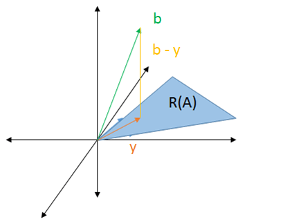
Since we're looking at `b - Aw`, let's instead consider only the vectors produced by doing `Aw`. The vectors that are formed by multiplying `A` with `w` are in the "range" of `A`, denoted `R(A)`.

Let's look at this visually. We'll start with the case when `A` is a `2xx2` matrix.

The matrix `A` can be represented as two vectors (the columns of `A`)

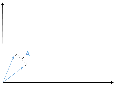
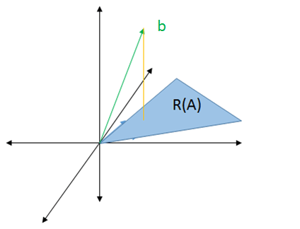
The range of `A`, `R(A)`, is the shaded area in blue between the vectors of `A` (this comes from the fact that the range of `A` is the span of the columns of `A` i.e., the column space of `A`)

If `b` lies in the shaded region, then `Ax = b` (which means we can find an `x` that satisfies that equation.) If `b` doesn't lie in the shaded region, then it is impossible to find an `x` such that `Ax = b`.

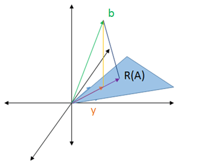
In the least squares problem, `A` has more rows than columns, so let's say it is `3xx2`.

So for `Ax = b`, since `A` only has `2` columns, `x` must have `2` rows and `b` must have `3` rows. This means that we must somehow find an `x` in `2` dimensions to reach a `b` in `3` dimensions. This is why we can't solve the least squares problem perfectly, as mentioned at the beginning.

The best we can do is to find the solution in `2` dimensions that is as close as possible to `b` in `3` dimensions. This can be done by dropping a straight line down to the `2` dimension area.

The solution, denoted by `y`, is the vector pointing to where the line drops. That line is a vector representing the difference between `b` and `y`.

This would be the vector in `2` dimensions with the shortest distance to `b`. We could choose any other vector and it would be farther to `b` than `y`.

That could be seen by looking at right triangles.

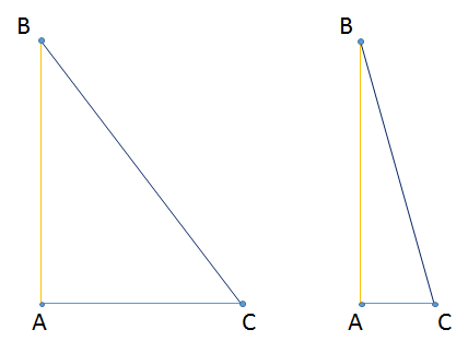
No matter what we choose for point `C`, the distance from point `A` to `B` will always be shorter than the distance from point `B` to `C`.

Going back to the statement before all the visuals, solving the least squares problem means making `norm(b-y)_2` as small as possible. From the visuals, we see that it is as small as possible when we take the vector pointing to the straight line dropped from `b`. The straight line is perpendicular to `R(A)`. More formally:

It turns out that `R(A)^(bot) = N(A^T)`, the null space of `A^T` (i.e., all the vectors `x` such that `A^Tx = 0`). So:

This leads to the final statement about the least squares problem: `x` solves the least squares problem for `Ax = b` if and only if `(A^TA)x = A^Tb`.

`QR` Decomposition (by Reflectors)

From `(A^TA)x = A^Tb`, we could theoretically do `x = (A^TA)^(-1)A^Tb`. But then we would be back again at the very beginning of this whole story. Because taking inverses of matrices is bad, we're gonna instead find a more efficient way to solve this problem.

Similar to the Cholesky decomposition, `QR` decomposition breaks `A` into `2` matrices, namely, `Q` and `R`. If `A` is an `n xx m` matrix where `n > m`, then `A = QR` where `Q` is an `n xx n` orthogonal* matrix and `R` is an `n xx m` matrix. Specifically, `R = [[color(blue)(hat(R))],[color(red)(0)]]` where `hat(R)` is an `m xx m` upper triangular matrix.

Recall that solving the least squares problem involves minimizing `norm(b - Ax)_2`. Since `Q` preserves length, we can do:

`Q^T` is an `n xx n` matrix and `b` is an `n xx 1` vector, so `Q^Tb` will be some `n xx 1` vector. We can say that `Q^Tb = [[color(blue)(hat(c))],[color(red)(d)]]`, where `hat(c)` is an `m xx 1` vector and `d` is an `(n-m) xx 1` vector.

`R = [[hat(R)],[0]]`, so `Rx = [[hat(R)x],[0]]`.

Combining these two points, we get:

Since the `2`-norm is a sum, we can break it up:

So from all of that, we get `norm(b - Ax)_2 = sqrt(norm(hat(c) - hat(R)x)_2^2 + norm(d)_2^2)`. We're trying to minimize `norm(b - Ax)`, which is the same as minimizing `sqrt(norm(hat(c) - hat(R)x)_2^2 + norm(d)_2^2)`. That happens when `norm(hat(c) - hat(R)x)_2^2 = 0`. That happens when `hat(R)x = c`. `hat(R)` is `m xx m` and `c` is `m xx 1`, so this problem is solvable using the techniques earlier in the story. `hat(R)` is actually upper triangular, so we can use back sub to solve for `x`. By solving for `x`, we are able to make `norm(c - hat(R)x) = 0`. What we are left with is `sqrt(norm(d)_2^2) = norm(d)_2`. That is the measure of the error in our solution (because we can't solve the least squares problem perfectly).

So if we're given `A`, how do we find the `Q` and `R`? Notice how the problem went from `Ax = b` to `Rx = Q^Tb`. That means that doing a `QR` decomposition invovles turning `A` into `R`.

That is, we want to find a `Q` such that `Q^TA = R` (since `A = QR`). We want to find some matrix that turns the first column of `A` into a vector with only `1` number in the first entry and so on.

It turns out that, for a vector `x`, there exists an orthogonal matrix `Q` such that `Q^Tx = [[-tau],[0], [vdots], [0]]`. So for each column of `A`, we can find a `Q_i` to do what we want.

For `m` columns of `A`, we would have `Q_m^TQ_(m-1)^T...Q_1^TA`. Then `Q^T = Q_m^TQ_(m-1)^T...Q_1^T`.

It turns out that `Q = I - 2u u^T` where `u = (x - y)/norm(x-y)_2`. `I` is the identity matrix. `x` is the column vector we're trying to change and `y` is the column vector we're trying to get. Doing the `QR` decomposition this way is known as doing it with "reflectors", where `Q` is the reflector.

Once we know what `Q` is, we are able to find `R` from `A = QR => R = Q^TA`.

Singular Value Decomposition

"This is the single most important thing in all of matrix analysis." -Professor Alex Cloninger

`QR` decomposition only works in some situations*. A more powerful method that works in all(?) situations is singular value decomposition (SVD).

Let `A` be an `n xx m` matrix with rank `r`. Then `A = USigmaV^T` where:

Assuming we know the values of `v_i`, how do we find the values of `sigma_i` and `u_i`?

It turns out that:

To get `sigma_i`, we can look at `(A^TA)v_i`:

So we get `A^TAv_i = sigma_i^2v_i`. This means `sigma_i^2` is an eigenvalue of `A^TA`. That means all `sigma_i` are the square roots of the eigenvalues of `A^TA`. To find the singular values `sigma_i` of `A`, we find the eigenvalues of `A^TA` and take the square root of them.

Since we have `Av_i = sigma_iu_i`, we can divide both sides by `sigma_i` to get `u_i`:

Besides being used to find the decomposition of `A`, `sigma_i` is important in another way. We've looked at `norm(A)_2` but only when `A` was a square matrix. Here, `A` isn't a square matrix, so the norm is a bit different. It turns out that `norm(A)_2 = sigma_1`.

Singular values are also helpful with finding the condition number of a non-square matrix. For a square matrix, the condition number was defined as:

However, non-square matrices don't have an inverse. So that definition of condition number doesn't make sense in this situation. We also defined condition numbers as:

Here, the maximum `A` can stretch a vector is `sigma_1` and the minimum `A` can stretch a vector is `sigma_m`.

And the condition number for non-square matrices is a measure of how good the least squares approximation will be.

In general, when we use the determinant method to find the eigenvalues of a `2 xx 2` matrix, we end up with a quadratic equation (`ax^2 + bx + c = 0`). For `3 xx 3`, we end up with a cubic equation. For `4 xx 4`, we end up with a quartic equation. It is always possible to find the roots of those equations. But for polynomials with degree greater than `5`, there are no formulas for finding the roots. This means the determinant method won't always work for matrices `5 xx 5` and greater.

That would mean that SVD decomposition would only work if `A^TA` was smaller than `5 xx 5`. This isn't true however. So we have to look at another way to find an eigenvalue.

Power Method

First, some terminology. `(lambda, v)` is an eigenpair of `A` if `Av = lambdav`. If `A` has eigenpairs `(lambda_i, v_i)`, then, by convention, we order them such that `abs(lambda_1) > abs(lambda_2) > ... > abs(lambda_n)`. `lambda_1` is considered the dominant eigenvalue.

Not only does the determinant method not work for big matrices, it only gives us the eigenvalues. We have to do a completely different method to find the eigenvectors. The power method gives us both the eigenvalues and eigenvectors (eigenpairs) at the same time. (The power method actually gives us the dominant eigenvalue. Variations of the power method give us all the eigenvalues.)

There is a restriction for the power method though. It only works when `A` is semisimple, i.e., all the eigenvalues are distinct.

So how does it work? Let's pick a random vector `q`. We can rewrite `q` in terms of the eigenvectors of `A`:

Now, let's multiply `q` by `A`:

Repeatedly multiplying by `A` results in:

Factoring out the `lambda_1^k`, we get:

When `k` gets large enough, then `A^kq ~~ lambda_1^kc_1v_1` (since `abs(lambda_1)` is greater than `abs(lambda_i)`, `lambda_i/lambda_1` will be less than `1` and with repeated multiplications, will get to `0`.)

Then we have:

This gives us a way of finding the eigenvector. How large will `k` be before we get a good estimate? If we let `q^((k)) = (A^kq)/lambda_1^k`, then we can look at `norm(q^((k))-c_1v_1)_2`:

So `norm(q^((k)) - c_1v_1)_2 le abs(lambda_2/lambda_1)^k sum_(i = 2)^n abs(c_i)norm(v_i)_2` goes to `0` as `k -> oo`. This means that we should stop when `abs(lambda_2/lambda_1)^k` is really small.

This says that repeatedly multiplying `q` by `A` and dividing by `lambda_1` will eventually give us the eigenvector `v_1`. It also says that if `abs(lambda_2/lambda_1)` is much smaller than `1`, then it won't take long for this method to converge (i.e. `k` will be small). But if `abs(lambda_2/lambda_1)` is close to `1` (i.e., `lambda_2` is close to `lambda_1`), then it will take a long time to converge (i.e., `k` will be large).

We have a way of finding the eigenvector, but it is dependent on the eigenvalue. And we currently don't know the eigenvalue. It turns out that we can't really compute it exactly, so we make an educated guess as to what it could be.

Inverse Power Method

The power method gives us one eigenvalue, namely the dominant one. But we still need to find the rest of the eigenvalues. It turns out that if `(lambda,v)` is an eigenpair of `A`, then `(1/lambda,v)` is an eigenpair of `A^(-1)`. This allows us to find the smallest eigenvalue of `A`. If `lambda^(text(*))` is the largest eigenvalue of `A^(-1)`, then `1/lambda^(text(*))` is the smallest eigenvalue of `A`.

Shift-and-Invert

So we have the largest and the smallest eigenvalues of `A`. But we still need the rest. It turns out that if `(lambda,v)` is an eigenpair of `A`, then `(lambda-rho,v)` is an eigenpair of `A - rhoI`.

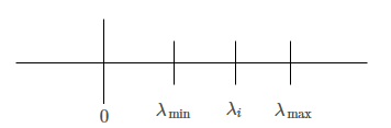
We can shift the interval down by `rho` to get:

Now, `lambda_i` is the smallest eigenvalue and we can use the inverse power method to get the eigenvalue of `A`. Doing the inverse power method on the shifted `A` would result in the largest eigenvalue, `lambda`, of `(A-rhoI)^(-1)`. Then `1/lambda` would be the largest eigenvalue of `A-rhoI`.

For the inverse power method and shift-and-invert methods, we've been calculating the inverse of `A` to perform the methods. As mentioned at the beginning of the story, inverting a matrix is a relatively time-consuming process. There's a better way to solve for `q^((j))`:

We know what `A - rhoI` is and we know what `q^((j-1))` is. In fact, this is the same `Ax = b` problem this whole story is about. (In the note before the Power Method section, I mention that `A` in these past three sections is referring to `A^TA` or `A A^T`. So here, `A` really is a square matrix.) `A - rhoI` is probably not positive definite, but it likely has a `LU` decomposition. Then we can write `A - rhoI` as `LU` to get:

Then we can use forward and back sub to get the values for `q^((j))`, which is relatively faster. This allows us to compute `L` and `U` one time and store them to make future calculations faster.

It turns out that if `A` is triangular, then `A - rhoI` is also triangular. Then `(A - rhoI)q^((j)) = q^((j-1))` can be solved mmediately with forward/back sub without having to find the `LU` decomposition.

Computers actually go about this by turning `A` into a tridiagonal matrix by using reflectors (from the `QR` Decomposition section), because forward/back sub with a tridiagonal matrix is really fast. Reflectors turn a vector into another vector with numbers on the top and `0`s on the bottom. So reflectors can be used to turn the columns of `A` into a vector with `3` numbers on top and `0`s on the bottom: